Using height and weight to predict heart disease
Which one would you choose?
| Option 1 | Option 2 |
|---|---|
 |
 |
Again
| Option 1 | Option 2 |
|---|---|
 |
 |
And now this
| Option 1 | Option 2 |
|---|---|
|
|
| William of Ockham | A problem-solving principle |
|---|---|
 |

How does that apply to Machine Learning?
- Using example of risk of heart disease with weight and height as input variables
- Let us look at the generation of the problem
Step 1: Mother nature generates some data
In [138]:
X = np.vstack([np.random.uniform(-1,1,500),np.random.uniform(-1,1,500)]).T
plt.xlabel('Height (cms)'),plt.ylabel('Weight (kgs)'),plt.xticks([]), plt.yticks([]),plt.tight_layout()
f = plt.scatter(X[:, 0], X[:, 1])

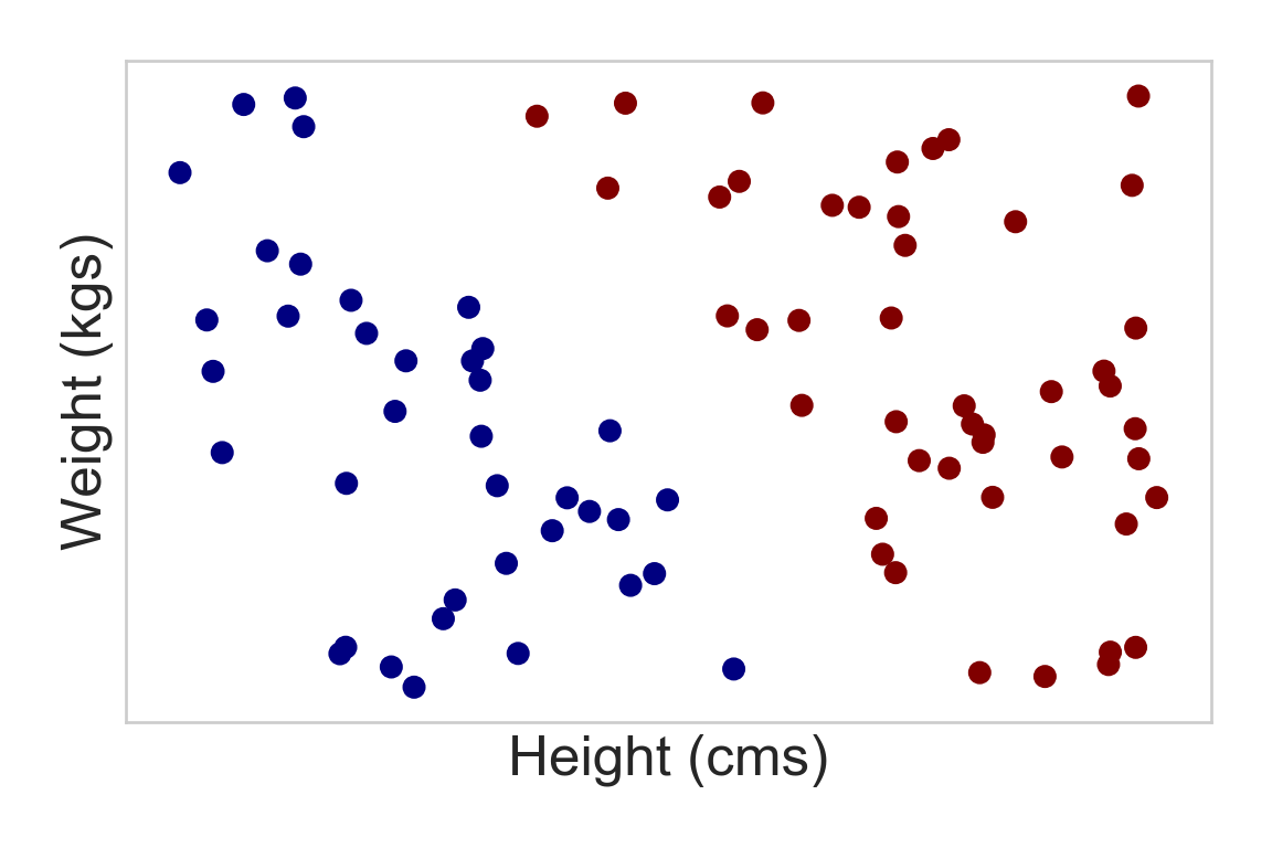
Step 2 - Mother nature labels the data
In [140]:
plt.xlabel('Height (cms)'),plt.ylabel('Weight (kgs)'),plt.xticks([]), plt.yticks([]),plt.tight_layout()
f = plt.scatter(X[:,0],X[:,1],c=y.flatten(),cmap=cm_bright)

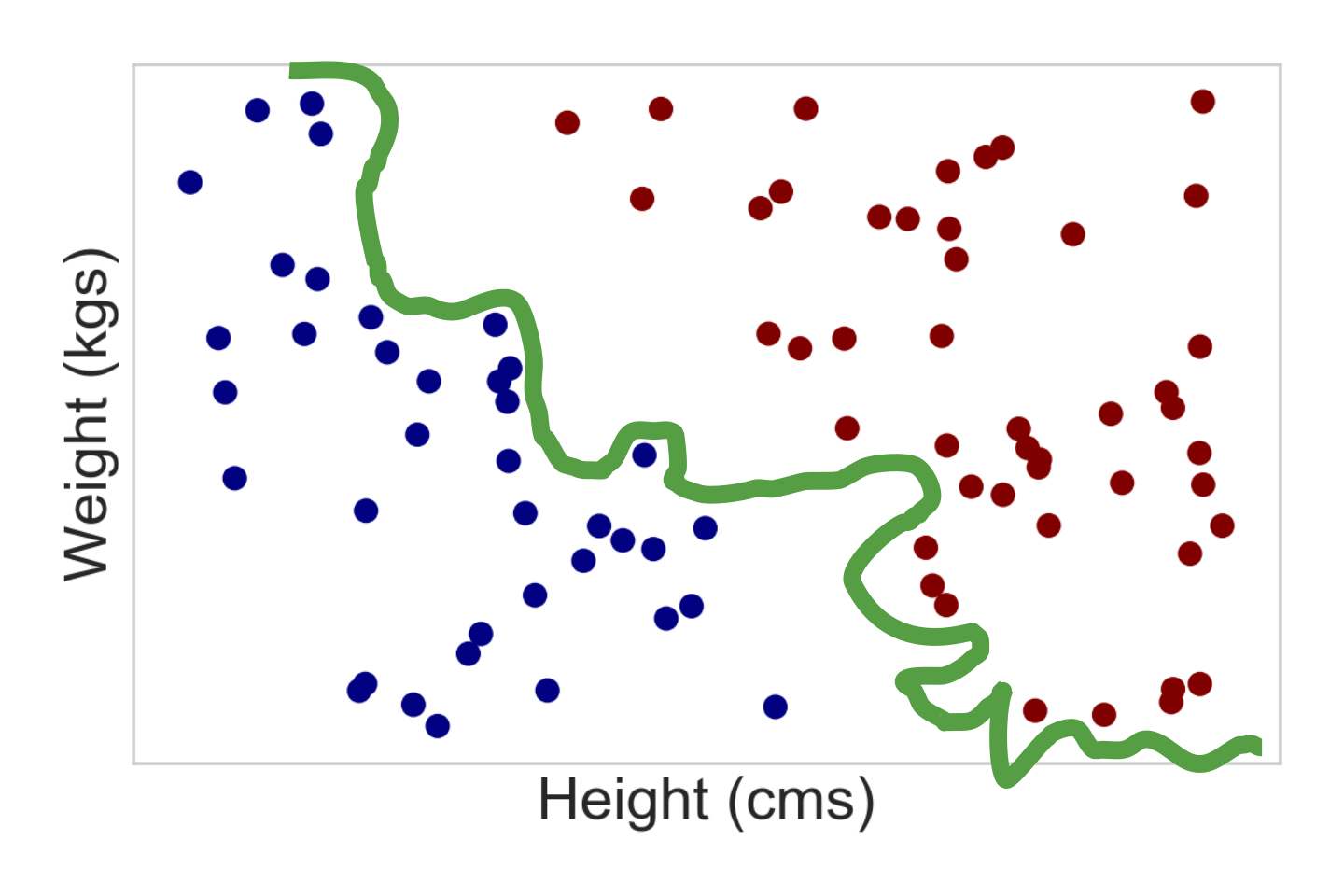
Step 3 - Mother nature gives us the training data
In [142]:
plt.xlabel('Height (cms)'),plt.ylabel('Weight (kgs)'),plt.xticks([]), plt.yticks([]),plt.tight_layout()
plt.scatter(Xtrain[:,0],Xtrain[:,1],c=ytrain.flatten(),cmap=cm_bright)
plt.scatter(X[:,0],X[:,1],c='k',alpha=0.1)
Out[142]:

ML Task
- Learn/estimate the function that mother nature used to label the data (training)
- Apply it to unlabeled data (testing)
Strategy
- Make assumptions regarding the form of the labeling function
- E.g., it is a line or a neural network or a tree
- Learn the parameters of the model using training data
Typically by optimizing over an objective function
We can bring the training error to 0 (or pretty close to it)
- Neural networks (universal function approximators)
- Kernel Support Vector Machines
In [269]:
# plot data
fig = plt.figure(figsize=[12,5])
plt.subplot(121)
plt.scatter(X[:,0],X[:,1],c=y.flatten(),cmap=cm_bright)
plt.subplot(122)
plt.scatter(trainX[:,0],trainX[:,1],c=trainy,cmap=cm_bright)
Out[269]:

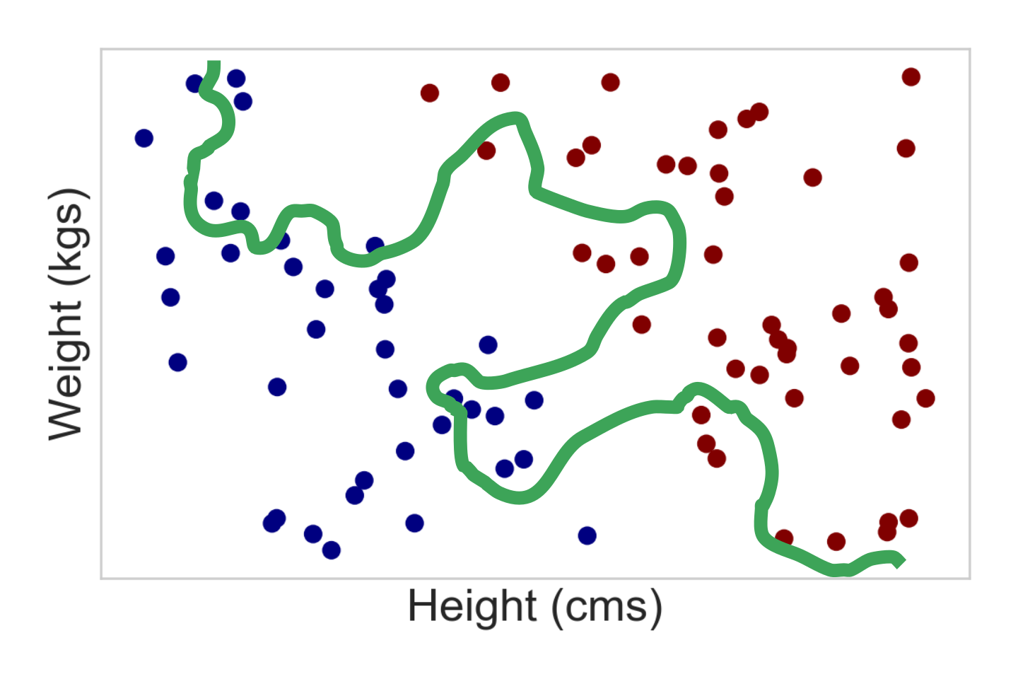
A neural network with 100 hidden units
In [275]:
ax = plt.subplot(111)
plotBoundary(trainX,trainy,clf,ax)
plt.title('Training Data. Mistakes = %d of %d'%(trainMistakes,len(trainy)))
Out[275]:

We can bring the training error to 0 (or pretty close to it)
- Neural networks (universal function approximators)
- Kernel Support Vector Machines
But should we?
Low training error does not guarantee a low true error
- Also called empirical risk vs. true risk
In [276]:
fig = plt.figure(figsize=(12,5))
ax = plt.subplot(121)
plotBoundary(trainX,trainy,clf,ax)
plt.title('Training Data. Mistakes = %d of %d'%(trainMistakes,len(trainy)))
ax = plt.subplot(122)
plotBoundary(X,y,clf,ax)
plt.title('All Data. Mistakes = %d of %d'%(allMistakes,len(y)))
Out[276]:

Complex models mean unstable models
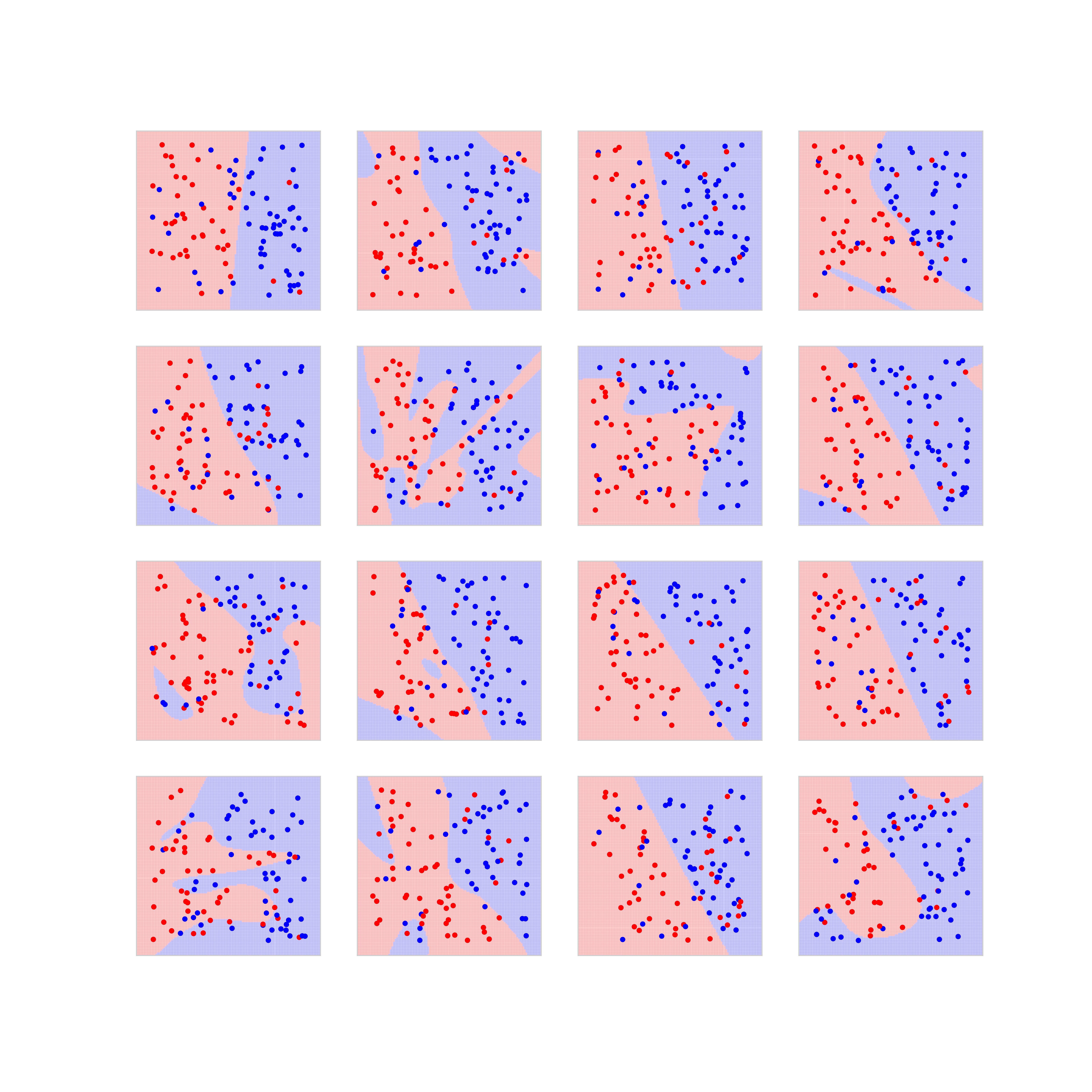
Applying Occam's Razor
- Option 1: Use a simpler model
- Option 2: Force your complex model to be simpler (regularization)
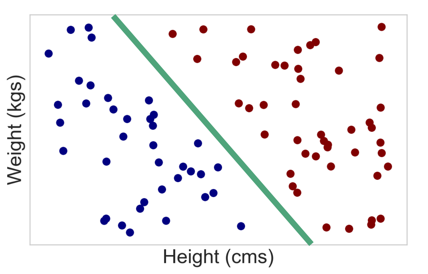
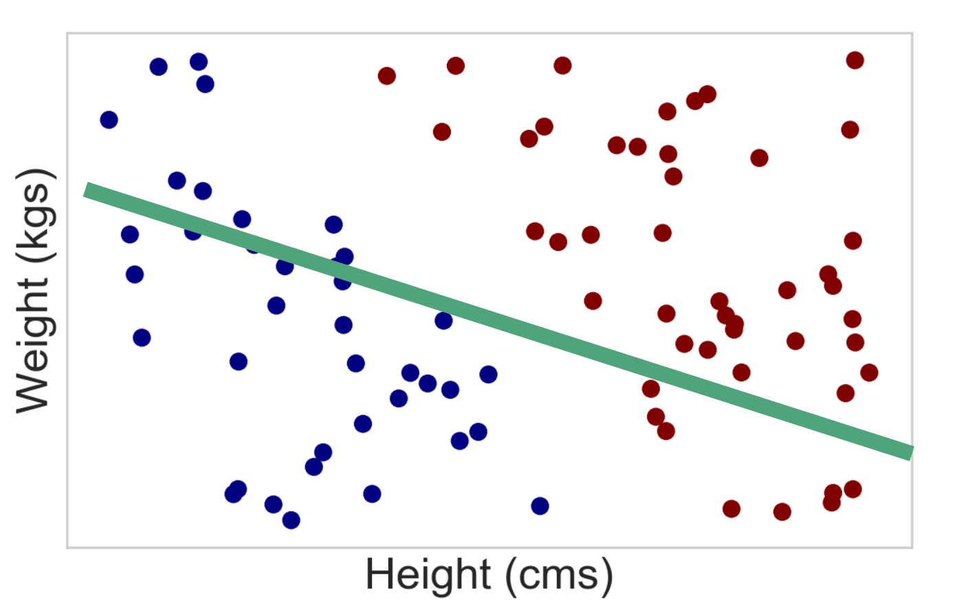
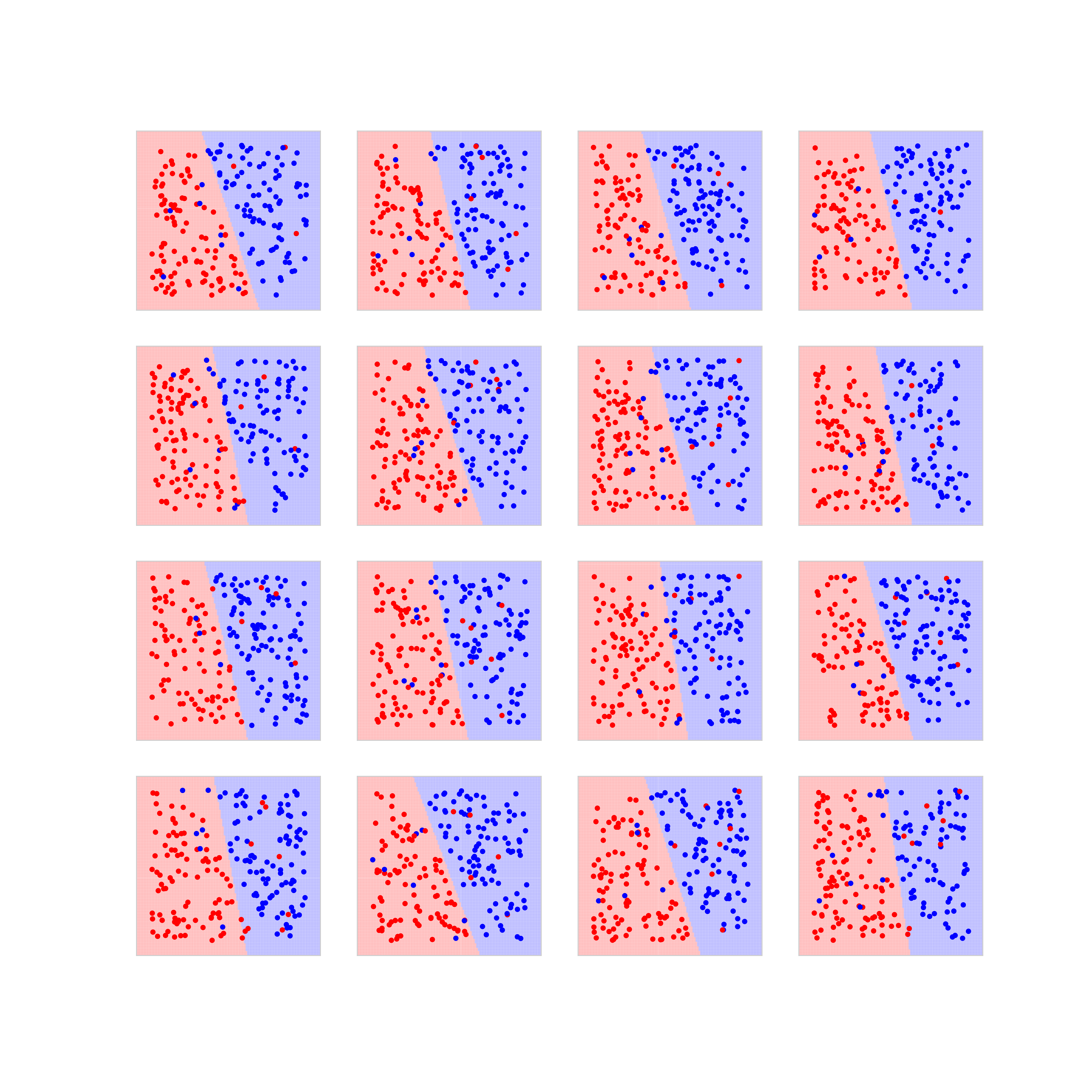
Using a linear classifier
In [287]:
fig = plt.figure(figsize=(12,5))
ax = plt.subplot(121)
plotBoundary(trainX,trainy,clf,ax)
plt.title('Training Data. Mistakes = %d of %d'%(trainMistakes,len(trainy)))
ax = plt.subplot(122)
plotBoundary(X,y,clf,ax)
plt.title('All Data. Mistakes = %d of %d'%(allMistakes,len(y)))
Out[287]:

Simpler models mean stable models
References
- The Role of Occam’s Razor in Knowledge Discovery