COMPAS dataset

This page contains a quick overview of a dataset that we will use often in this course. We also use to do a walkthrough of the ML pipeline.

Under Construction

This page is still under construction. In particular, nothing here is final while this sign still remains here.

A Request

I know I am biased in favor of references that appear in the computer science literature. If you think I am missing a relevant reference (outside or even within CS), please email it to me.

Background

In 2016, ProPublica published an article titled Machine Bias , which studied a software called COMPAS that was used to predict recidivism . It showed a bias against black defendants when compared to white defendants:

Both the article as well as the accompanying article has more details on how they came to the above conclusion. In short, here is what happened. Broward County, Florida was using COMPAS scores in pre-trial release decisions. ProPublica got the COMPAS score from the county via a public record request-- these scores predict the likelihood of a defendant committing a crime in the future. Then via public criminal records from the county , ProPublica figured out which of the defendants actually went on to commit a crime in the next two years and compared those with the COMPAS scores and did a bunch of statistical analyses (see the accompanying article for more details).

The ProPublica article is considered a landmark article especially within folks who study algorithms and its interactions with society. Further, the COMPAS dataset created by ProPublica has been used in many analyses and courses (and indeed, we will also use the dataset). I encourage y'all to read the above articles just to get a sense of how the ProPublica investigation was done.

A Rejoinder

There has been some push-back against the ProPublica analysis. In particular, the work of Flores et al. showed that the COMPAS tool is fair in the sense that it is well "calibrated" (which is also a natural notion of fairness). While this seems contradictory to the ProPublica investigation, we will come back to these diverging analyses when talking about fairness in algorithms. In particular, we will show both of the analyses are correct and further, such contradictory conclusions are inevitable in a very strong mathematical sense.

A walkthrough the ML pipeline

We first recall the ML pipeline we will study in this course, which we saw earlier:

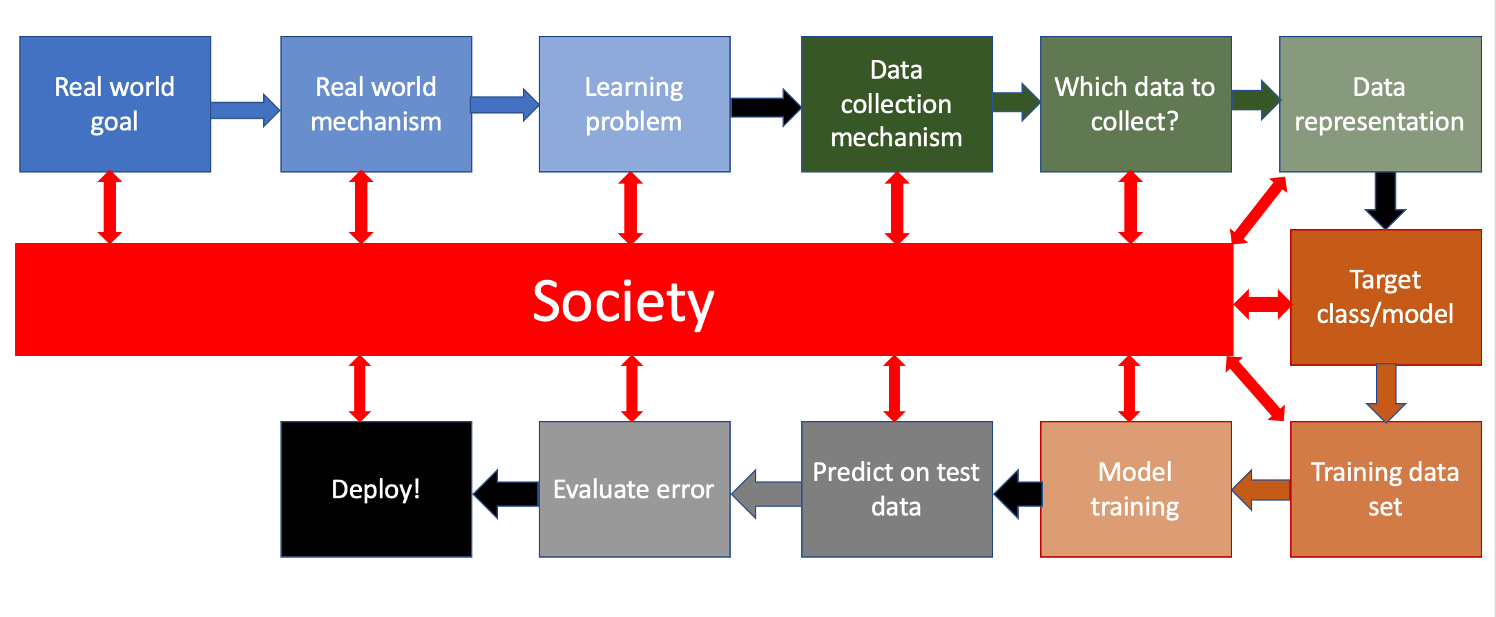
In these notes we will consider a (made-up) scenario related to the COMPAS dataset so that we can illustrate what each step of the ML pipeline (where for now we will essentially ignore its interactions with society) in this context.

The Problem

Imagine a situation where the creator of COMPAS had access to the COMPAS dataset. In particular, you are in the team that wants to predict recidivism based on the COMPAS dataset. How would you go about doing it?

Well, let's just walk through the ML pipeline to see how you would go about doing this.

Below we will walk through all the labeled steps in the ML pipeline and try to address how each step would work in the above scenario. However, we will "define" each step at a high level with the understanding that we will address technical details of each step in future lectures.

Real world goal

This is the step where you (or someone else) decides the high level problem being solved.

Actually, your group was handed the problem to predict recidivism and this step is something that preceded your involvement (aka "above your pay grade"). However, there would be situations where you (or someone else making this decision) have to answer this question. (And even if you were not involved in this step, it would help you come up with a better solutions if you knew what the real world goal was.) Let us assume that the following was the overall goal:

Real world goal

Reduce crime in society.

Note that the above goal is very vague-- in the sense that it is not very specific about how one would go about "reducing crime." However, this is how original real-life problems are formulated-- they are not very prescriptive (or indeed very precise). This then brings us to the next step.

Real world mechanism

Once you have defined your real life problem you will need to solve it in the real world. This means you (or someone else) needs to decide what real life process or mechanism you will use to ground the high level problem in reality. After this step, the real life goal should be more "actionable" now. Note that this mechanism need not be something that is already well-established and could be something that your group might need to build but it should be something concrete that the mechanism, if need be, can be implemented/created in the real world.

Again this step was "solved" before your group was handed its project. Again, there would be situations where you (or someone else making this decision) have to answer this question. Let us assume this was the thought process:

Real world mechanism

Based on some studies (or not!), your superiors decided that repeat offenders contribute most to crime. This in turn they decided would mean that if one could identify who would commit a crime again in the future, then one could use this information when making judgment on the current crime. Thus, they decided they wanted a system that can identify folks who will re-offend in the future and then promptly handed off the problem to your group to solve it.

In the above decision, the real life mechanism was (i) hypothesizing that repeat offenders are a big reason for crime and hence (i) repeat offenders should be identifies. What was left unsaid is what happens after this identification. In this case, this identification could then be used by the established legal system to determine the length of sentence for a defendant who is identified to be someone who might re-offend.

Learning problem

Once you have decided on your real world mechanism, the next step is to figure out how to map the outcome of the mechanism to be something that (i) can be measured and (ii) then your goal is to figure out a way to "learn" or predict the outcome of the proposed mechanism.

This is the first step where your group will make a decision. The "higher-ups" have made the problem to identify defendants who will re-offend in the future. Of course, doing this without any error or with absolute certainty is not possible. So the best your group can come up with is to try and predict who will re-offend:

Learning problem

Your group decides on the simplest learning problem: given a defendant predict if they will re-offend or not (in other words you are doing binary classification (binary because you are "labeling" defendants as either going too re-offend or not going to re-offend and you are doing classification because you are putting people into the two bins-- i.e. giving them a binary label and hence assigning them a "class."

There is another related option (which is what COMPAS : instead of assigning defendants to two scores: they assign a score from $1$ (being least likely to re-offend) to $10$ (most likely to defends). This range of score (rather than a binary classification) could potentially be more useful to the end user of your system.

However, for our discussion (and indeed for most of the rest of the course), we will focus on binary classification.

More involved decisions

Above the decisions were relatively straightforward since there was a "target variable" (whether someone will re-offend or not) corresponding to the goal from the last step. However, in many case this map is not as straightforward. See Hal Duame III's blog post on the machine learning pipeline

An even more meta-question (which we will come to later in the course) is the following: Should you be solving the problem from the previous step as a learning problem at all? Or more generally is a computational solution the right thing to do?

Data collection mechanism

Now that you have defined your learning problem, you will need some data to train (as well as test) your model. But wait: how do you get the data in the first place? In particular, how is the data generated? In many cases you might not be able to do this because the data might be "given" to you. This step is then to decide on how your group is going to collect the relevant data.

In this particular example:

Data collection mechanism

Your group decides to use the COMPAS dataset.

However, it is a useful exercise to recall what mechanism ProPublica used to collect the data (see the accompanying article to the main ProPublica article for details). In short, they used the existing public records law to get some data and generated the rest of the data was generated via a public government website. An important point to note this is a very labor intensive process and it's not like writing a script to log certain information about a system (though that also can work as in Hal Duame III's blog post on the machine learning pipeline . In other words, generating data can be expensive (if not directly in terms of money then in person-hours).

Which data to collect?

After you have decided on how you are going to collect data, the next question if which data you are going to collect. Again, in many cases you might not be able to do this because the data might be "given" to you. In this particular example:

Which data to collect?

Your group decides to use whatever data the COMPAS dataset has.

However, it's worth it to note that in the ProPublica data collection, they could only collect data that was public and so your group does not have access to data that is not in the public domain that could be relevant to solve your learning problem. See the next callout for a pertinent example.

Measuring crime

We would now like to highlight one unavoidable (and potentially huge) issue with measuring/collecting data on when a crime was committed. For example, ideally in your group's problem you would like to figure out when someone re-offends: i.e. commits a crime again. However, public/police records can only show when someone was arrested for a crime. Keep this distinction in mind-- we will come back to this later on in the course (especially when we talk about feedback loops).

Data representation

Now that you have figured out how and which data to collect, you now have to figure out the format of the data to be collected. For example, if you want to collected data on age, do you record their age in years. Or do you collect years or months? Or do you collect the birthday (which you might not be able to do)? On the other side of the spectrum, do you just collected ranges, e.g. in 10 year ranges (i.e $0$ to $9$ years old, $10$ years to $19$ years old and so on). Or in some other format? Note that there is a tradeoff: collecting more detailed data might be better for your learning system but it could also be more expensive to collect more granulated data.

In this example:

Data representation

Since your group is using the COMPAS dataset, the data representation is also given to you.

Target class/model

In the introduction, we saw what is a model. Deferring the technical details for now, in learning problems, we restrict the class of models that we will aim to use to do our classification. However, there are multiple such classes so we need to decide on a "target" class of models.

This step is probably one of the most (if not the most) technical of all steps in the ML pipeline. We will spend a week covering some of the basic/well-known models used in machine learning. For this example, let us consider the simplest model:

Target class/model

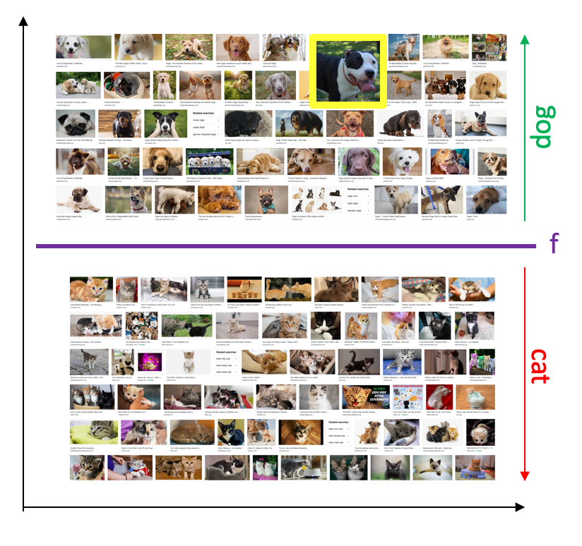
Let us assume that your group chooses a linear classifier. Again we will consider this model in more detail later on, but we have already seen (a made up) example of this when we were looking the classifying cats vs. dogs in the introduction :

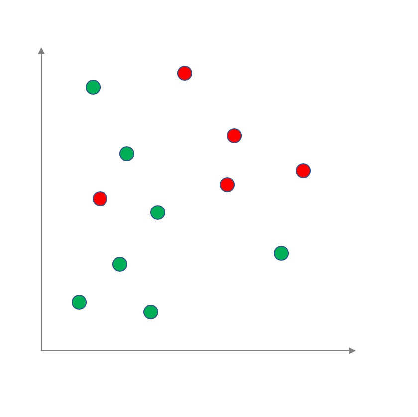
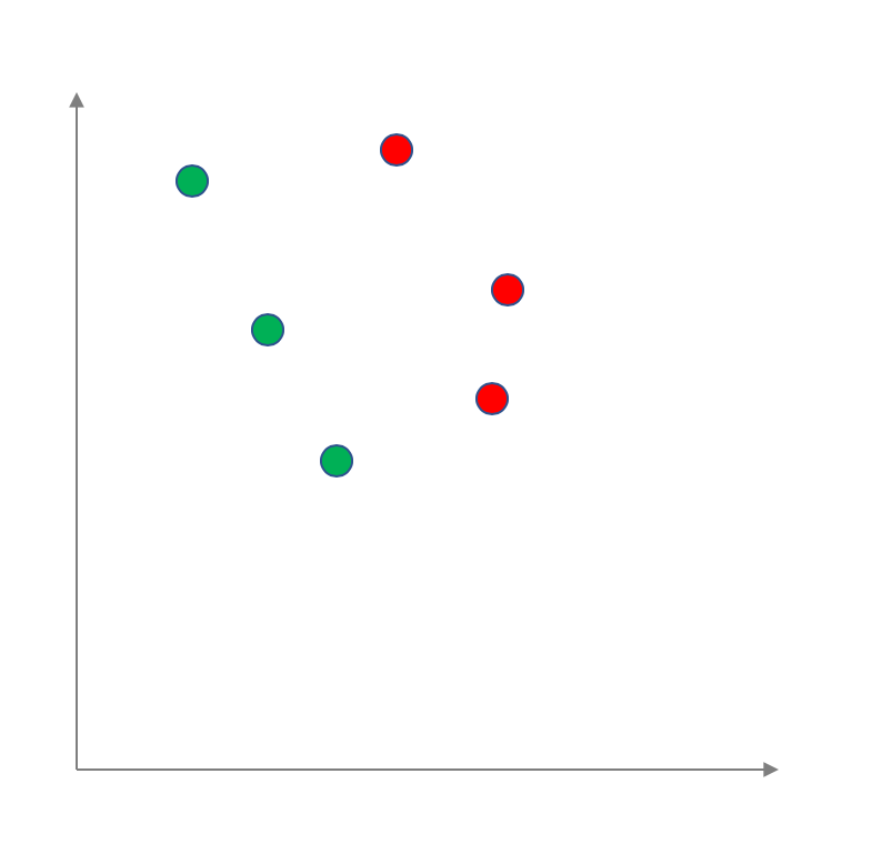
where we used a "line" to separate out the cat pictures and the dog pictures. Of course the above is a made up example in that we do not get such a clear distance between the positive and negative labels.

For simplicity let us assume that each data point has two numerical attributes. In other words it can be visualized as a 2D-plot with the green circles being the positive label and the red circles being the negative labels:

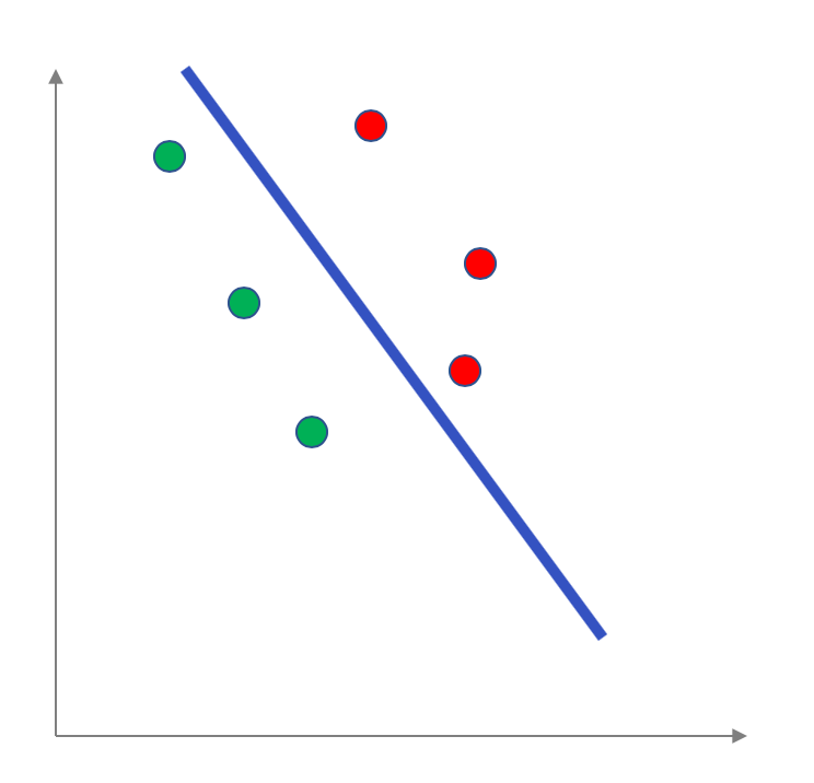
It turns out that a linear model for data with two attributes is literally a line that separates the points into a "positive" half and into a "negative" half. For example for the above example, here is a linear model (the blue line):

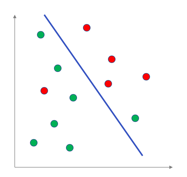
In fact, the blue linear model is the best possible one in the sense among all the lines that separate the set of points the blue one is the one with fewest errors (or mis-classifications)-- i.e. number of points whose true label does not match with the label assigned to the point by the model.

It turns out for data with more attributes, we can map the data points to a higher dimensions and then a linear model is a generalization of a line to higher dimensions: the hyperplane . More on this later on in the course.

Training dataset

So you have figure out the model you are going to use and you have access to a labeled dataset (COMPAS dataset). What you would like to do is to figure out a good model from this dataset. We will address the step of converting labeled data into a model in the next step but one option is to use all of the labeled dataset to generate the model. However, this creates the following potential issue.

Generalization

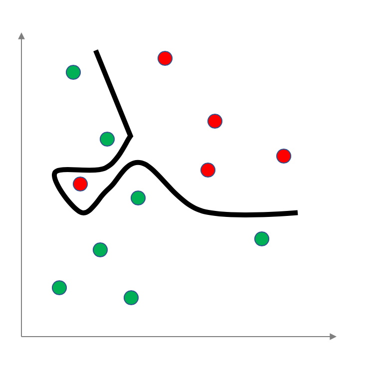
At best the labeled data set will be an approximation of the "ground truth"-- this means that there could exist patterns that are specific to the given dataset that do not exists for the actual ground truth. Then when you learn a model on this dataset this pattern might get "baked" into the model, which when applied later on to input "from the wild" could lead to problematic classification. This is know as overfitting . In the context of the made up example above, here is an example of overfitting the given labeled data (note that here we are not using a linear model to separate out the positive and negative data):

One common way to handle this is to only use part of the dataset to train the model (and hence, this chosen part of the dataset is called the training dataset) and use the rest (or the whole dataset) to measure measure overall error. One might repeat this process a few times and then somehow aggregate the various models generated. E.g. one could pick the model with the smallest overall error (though there are other possibilities). For this example:

Training dataset

Your group decides to pick a random $50\%$ of the dataset as the training dataset. For example, the sampled training dataset for the example above could look like this:

Model training

Once we have figured out the training dataset and out target model class, the next step is to figure out the "best" model from this target class that best "explains" the training dataset.

This step of the ML pipeline is probably the most mathematically involved when compared to the other steps (there is some beautiful math in there though!) so we will mostly avoid talking about this in detail. We will talk about this step in bit more detail later on in the course but for now

Model training

Assume that your group has access to a blackbox that figures out the best possible model that separates the positive and negative data points in your training set. E.g. here is what the learned linear model on the above training set will look like:

Predict on test data

Now that you have your model that was learned, you have to figure out a test dataset to evaluate how good (or bad) your learned model is. We will leave the evaluation to next step but given a model it is easy to figure what the label of a datapoint in the test dataset will be (for linear model its just a matter of figuring out which side of the line the test datapoints lie on). There are various possibilities here but here is the obvious one:

Predict on test data

Your group decides to pick the $50\%$ of the original dataset that was not included in the training set, i.e. (below we leave the learned linear model in the plot):

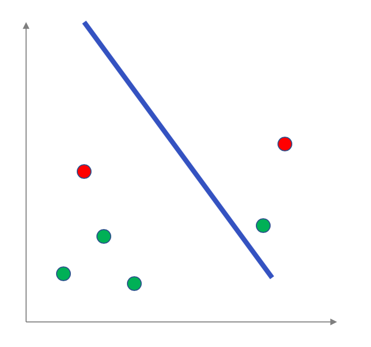
Note that everything below the line is considered to be labeled positive and everything above the line is considered to be labeled negative (so in particular, the red point below the line and the green point above the line are not classified correctly).

Evaluate error

Now that we have used our learned model to predict the labels in the test dataset we need to evaluate the error. Again, there are multiple mathematically precise measures of evaluating error. For this example, we will again go with the obvious one:

Evaluate error

Your group decided to calculate the percentage of points in the testing dataset that were mis-classified. So in the example above:

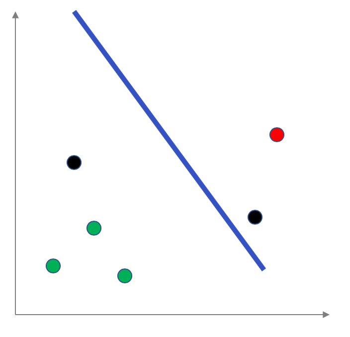
The mis-classified points are colored in black and so we have $2$ mis-classified points, which is an error rate of $\frac 26\approx 33\%$.

Deploy!

Now your group is ready to deploy the learned model. Or is it?

Independence of ML pipeline steps from the problem

You might have noticed that once we fix the data representation all of the remaining steps have procedures that are actually independent of the original problem you started off with. This is what makes ML powerful (since the same abstraction works in multiple scenarios) but also leads to pitfalls/blindspots (as we will see later in the course).

Next Up

In the next lecture, we will consider steps in the ML pipeline related to data collection.