Recitation 10
Recitation notes for the week of November 6, 2017.
Q2 on HW 7
We will talk about the problem in terms of examples.
Example 1
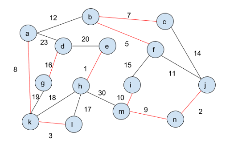
In this case $G$ is the following graph: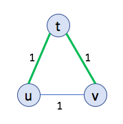
In the above graph an MST is shown with the green edges.
The input sets are defined as follows (note $n=2$ and $M=5$): \[S_u=\{1,2,5\},\] \[S_v=\{2,4\},\] \[S_t=\{2,3,5\}.\] The corresponding array representation will be \[A_u =[1,1,0,0,1],\] \[A_v =[0,1,0,1,0],\] \[A_t =[0,1,1,0,1],\]
Note that at the end, $t$ needs to know \[\{1,2,5\} \cap \{2,4\} \cap \{2,3,5\} =\{2\}\] or equivalently, \[B~~ =[0,1,0,0,0].\]
Note
Communication cost is $1\cdot 5 +1\cdot 5 =2\cdot 5=10$.
Example 2
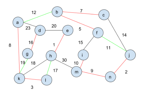
In this case $G$ is the following graph: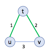
In the above graph an MST is shown with the green edges.
Consider the case when all the input sets are exactly the same as in Example 1. Thus, node $t$ needs to output $\{2\}$ (or equivalently $[0,1,0,0,0]$ as before).
Note
Communication cost is $1\cdot 5 +2\cdot 5 =3\cdot 5=15$.
Example 3
In this case $G$ is the following graph: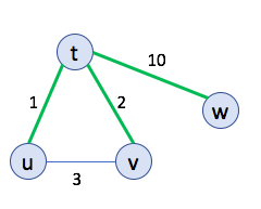
In the above graph an MST is shown with the green edges.
Consider the case when all the input sets $S_t,S_u,S_v$ are exactly the same as in Example 1. But we have another set now \[S_w=\{3,4,5\} \text{ or equivalently } A_u=[0,0,1,1,1].\] Thus, node $t$ needs to output $\emptyset$ (or equivalently $[0,0,0,0,0]$).
Note
Communication cost is $1\cdot 5 +2\cdot 5 +10\cdot 5 =13\cdot 5=65$.
Some important clarifications on what the algorithm can do and cannot do
- Your algorithm can use the knowledge of $G$ to figure out the protocol. In all of the above examples, the algorithm use the knowledge of $G$ figure out which edges would be used to transmit bits over (they happened to be the edges of an MST of $G$).
- Once the protocol is decided, only then do the sets ($A_u$ for $u\in V$) come into the picture.
- The protocol tells at any point of time $t$ what the node $u$ should do. In particular, based on its input $A_u$ and all the bits it has received up to time $t-1$, it needs to decide what bits to send at time $t$ to each of its neighbors.
- Multiple bits can be sent on an edge $e$ at the same time.
- If during the run of the entire protocol, edge $e$ sends $b_e$ bits in total, then the total cost incurred on sending these $b_e$ bits will be $b_e\cdot c_e$.
- At the end of the protocol, node $t$ has to output the final answer based on its input $A_t$ and all the bits it received from all its neighbors over the entire run of the protocol.
Boruvka’s Algorithm
This is another algorithm to find the minimum spanning tree for a graph with distinct edge weights (none of the edges have the same value).
Algorithm Idea
The goal of the algorithm is to connect "components" using the shortest edge between components. It begins with all of the vertices considered as separate components and then continues till there is one connected component left (which can be proven is an MST).
Next we present the Algorithm Details, courtesy of Wikipedia .
Algorithm Details
                            //Input: A connected graph G whose edges have distinct weights

                            Initialize a forest T to be a set of one-vertex trees, one for each vertex of the graph.

                            while T has more than one component:
                                for each component C of T:
                                    Let S be an empty set of edges
                                    for each vertex v in C:
                                        Find the cheapest edge from v to a vertex outside of C, and add it to S
                                    Add the cheapest edge in S to T
                                Combine trees connected by edges to form bigger components

                            return T // The set of edges in T forms the MST of G
Note
An edge can be selected twice (by two different components). This is fine.
Example 4
We consider the run of the Algorithm on the following graph:
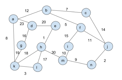
- Initially all the vertices themselves form their own component.
- In the first iteration of the
whileloop, all the red edges are picked and added toT:
 .
. - In the second iteration of the
whileloop, all the green edges are picked and added toT:
 .
. - At this point, we are done.
There are two more examples on the Wikipedia page .
Complexity
Note that the while loop will halve the number of components each time. We start with $n$ components (the number of vertices), so the while loop runs at most $\log{n}$ times. In each iteration of the loop, we look through the edges, taking $O(m)$ time. Thus, overall we have $O(m \log{n} )$ time.
Correctness
Proof Idea
As in class we consider the case when all the edge costs are distinct. Then note that the algorithm in each iteration of the while loop, add the cheapest crossing edge for the cut $(C,V\setminus C)$ for every (non-empty) component $C$. Thus, by the cut property lemma, this is a "safe" choice.
After each addition of an edge, the algorithm creates a forest in the original graph. As, we just argued, this forest does not have any edges that would not be in all MSTs. Finally, the algorithm runs until there is only one component. Recall from the sample problem on HW 4, a forest with one component is a tree.
Recurrence Relations
Many, if not most, of the divide and conquer algorithms that we will study in this class, will recursively call on $q$ subproblems of size $n/2$ each and combine results in linear time (think merge sort, which has $q=2$). Then the immediate question is:
The textbook (especially Section 5.2 has the details) answers this. We have the following result:
Theorem
Define $T(n)$ as follows. For some constant $c$, \[T(n) \le q\cdot T(n/2) +cn\] when $n>2$. Otherwise we have \[T(2) \le c.\]
Then we have the following results:
- $q=1$: \[T(n) \text{ is } O(n).\]
- $q=2$: \[T(n) \text{ is } O(n\log{n}).\]
- $q>2$: \[T(n) \text{ is } O\left(n^{\log_2{q}}\right).\]
The case of $q=2$ was proved in class. For the proof of the other cases, see the textbook.
Further Reading
Section 5.2 in the textbook.