Recitation 11
Recitation notes for the week of November 13, 2017.
Recurrence Relations
$T(n) = T(n/2)+O(1)$
We start off with the Binary search algorithm (stated as a divide and conquer algorithm):
Binary Search
                                        // The inputs are in A[0], ..., A[n-1]; v

                                        l = 0
                                        r = n-1
                                        return binary_search(A,l,r,v)

                                            # Recursive definition of Binary Search
                                            binary_search(A,l,r,v)

                                                if l == r:
                                                    return v == A[l] # Return 1 if A[l]=v and 0 otherwise
                                                else:
                                                    m = (l-r)/2
                                                    if v <= A[m]:
                                                        return binary_search(A,l,m,v)
                                                    else:
                                                        return binary_search(A,m,r,v)
Runtime Analysis
It is easy to check that every line except the recursive calls of binary_search takes $O(1)$ time. So if $T(n)$ is the runtime of binary_search, then it satisfies the following recurrence relation:
Recurrence Relation 1
\[T(n)\le \begin{cases} c & \text{ if } n=1\\ T(n/2)+c & \text{ otherwise }.\end{cases}.\]
Next, we will argue the following
Lemma 1
For recurrence relation 1 above, \[T(n)\le c\cdot (\log_2{n}+1).\]
Proof Idea
The idea is to unroll the recurrence. Each level has a contribution of $c$:
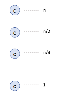
Since there are at most $\log_2{n}+1$ levels, this implies the claimed bound.
Proof Details
See Page 243 in the textbook.
Exercise 1 (do at home)
Prove the recurrence using the "Guess and werify (by induction)" strategy.
HW 8 Q2
Make sure you present a divide and conquer algorithm for part 2 on Q2 on HW 8 and and analyze it via a recurrence relation. Otherwise you will a 0 on all parts.
$T(n) = T(n/2) +O(n)$
We now consider the following recurrence relation
Recurrence Relation 2
\[T(n)\le \begin{cases} c & \text{ if } n=1\\ T(n/2)+cn & \text{ otherwise }.\end{cases}.\]
The book on Page 219 solves this recurrence. We do a very quick overview now.
We do the "unroll the recurrence and use the pattern technique." At an arbitrary level $j$, there is one instance, of size $\frac{n}{2^j}$ and contributes $\frac{cn}{2^j}$ to the recurrence relation. Thus, we have (for $n\ge 2$): \[T(n)\le \sum_{j=0}^{\log_2{n}} \frac{cn}{2^j} =cn\cdot \sum_{j=0}^{\log_2{n}} \frac{1}{2^j}.\]
Working out this geometric sum, we will find that it converges to $2$. Thus, we can say, for recurrence relation 2 above we have \[T(n) \le 2cn \le O(n).\]
Adversarial Lower Bound
The difference from previous lower bounds
- Lower Bounds Previously: Show the lower bound for a specific algorithm.
- Goal of Adversarial Lower Bound: Show lower bound for any correct algorithm that solves the problem.
The "game"
For adversarial lower bounds one can think of the whole process as a game with an adversary: i.e. one's opponent in a contest or dispute.
In particular, for the adversarial lower bounds, it is game between (an arbitrary) algorithm and the adversary:
- algorithm wants to compute the correct answer as quickly as possible.
- the
adversaryis trying to come up with input that will make algorithm take a long time (you should assume that theadversaryknows the code of the algorithm). - We want to show that
adversarycould force algorithm to do some amount of work which becomes the lower bound.
Theorem 1
Every correct algorithm that solves the problem of searching in a sorted list needs $\Omega(\log{n})$ time.
What makes the proof for Theorem 1 (and proving adversarial lower bounds in general) is that there exist algorithms that work well for the specific case and otherwise are $O(\log n)$ in general. We want to show that for every algorithm, there exists at least one input on which its runtime is $\Omega(\log n)$.
Note
The stuff below is copied from the support page on adversarial lower bounds.
Algorithms that work well on specific inputs
Let us fix any input $a_0,\dots,a_{n-1};v$. Let us first consider the case that $v$ is not any of the $a_i$'s. Then here is an algorithm that will solve this instance in $O(1)$ time:
Sseraching a non-existent value
                                        // The inputs are in A[0], ..., A[n-1]; v
                                                if(v> A[n-1] or v< A[0])
                                                        Output "v not found"
                                                else
                                                        Return the output of binary search
Couple of remarks are in order:
- First note that if we did not run binary search in line 5, then the above algorithm will not be correct. Of course we are only interested in proving lower bounds for all correct algorithms.
- Note that the above algorithm is not a counter-example to the Theorem because binary search is known to run in $\Omega(\log{n})$ so the algorithm like the binary search algorithm also runs in $\Theta(\log{n})$ time.
So what happens if indeed $v=a_i$ for some $i$? One can also come up with another algorithm that runs in $O(1)$ time for that specific case (and $O(\log{n})$ in general);
Searching a present value
                                        // The inputs are in A[0], ..., A[n-1]; v and v=A[i]
                                                if(v == A[i])
                                                        Output i
                                                else
                                                        Return the output of binary search
What the above algorithms make clear is that we cannot pick a "bad input" that is independent of the algorithm. In other words, we should try and pick the hard input based on the algorithm. One nice way to do this is via the so called adversarial argument.
An adversarial argument for the searching problem
We finally return to proving the Theorem. As you can surmise from the section heading, we are going to use the adversarial argument to do this. However, we will use it in a slightly different way than how it was used in the videos above. In particular, the general idea is as follows (which can be applied to other problems too):
Adversarial Argument to Bound Number of Input Accesses
Whenever the algorithm accesses a location in the input, the adversary fixes the value at that location (and potentially other values too). Any future access by the algorithm to any of the fixed values is given for "free". The goal of the adversary is to fix values in such a way so that there is always two ways to fix the unfixed values so that the algorithm on the two resulting inputs has to output different answers. Note that this implies that the algorithm cannot terminate. If the adversary is able to play this game long enough, then we have our lower bound.
Next we implement the above overall scheme to prove the Theorem.
Proof Idea
We will set $v=1$ and assume that all $a_i\in \{0,1,2\}$. The main idea is the following. Whenever the algorithm queries the position $j$ in the numbers $a_0,\dots,a_{n-1}$, the adversary sets either $a_j=0$ or $a_j=2$ depending on how many elements remain unfixed. (Note that since the numbers are sorted this might fix some other values.) In particular, we make sure that after each access the number of unfixed values is at least half of the previous number of unfixed values. Since the initial number of unfixed values is $n$, this implies that the algorithm has to make $\Omega(\log{n})$ accesses to the input. This is because if there are fewer access, there is at least one unfixed value, which could be either a $0$ or $2$ (in which case the algorithm has to output not found) or it can be $1$ (in which the algorithm has to report that $v=1$ is present).
Note to TA
Unless you have extra time, skip the proof details.
Proof Details
After the $i$th access by the algorithm to the values $a_0,\dots,a_{n-1}$, we define the interval $[\ell_i,r_i]$ to be the positions $j$ such that the adversary has not fixed $a_j$ yet. Before the first access we have $\ell_0=0$ and $r_0=n-1$. Further, we will maintain the following invariants:
- $a_j=0$ for every $j\in [0,\ell_i)$ and $a_j=2$ for every $j\in (r_i,n-1]$.
- $a_j$ for $j\in [\ell_i,r_i]$ has not been fixed.
- $r_{i+1}-\ell_{i+1}+1\ge \frac{r_i-\ell_i+1}{2}$ for every $i\ge 0$.
Before we show how the adversary maintains the above invariants, we assume that the adversary is able to do the above and finish our proof. Since $r_0-\ell_0+1=n$, as long as the number of accesses $i$ is at most $\log_2{n}-1$, the last invariant above implies that $r_i-\ell_i+1\ge \frac{n}{2^{\log_2{n}-1}} =2$. Then by the second invariant this implies that at least one $a_j$ has not been fixed and further from the first invariant it can be picked to be any value in $\{0,1,2\}$, which means the algorithm cannot terminate (since it cannot know for sure if $v=a_j$ for some $j$). This implies that the algorithm has to make at least $\Omega(\log{n})$ accesses, as desired.
Finally, we show how the adversary can maintain the invariants. In particular, let us assume by induction we have able to maintain the invariants for up to $i$ accesses. (Note that in the case case of $i=0$ we have $\ell_0=0$ and $r_0=n-1$.) Now consider the $(i+1)$th access-- let it be to the index $j$. If $j\not\in [\ell_i,r_i]$, then we set $\ell_{i+1}=\ell_i$ and $r_{i+1}=r_i$ (and so we do not fix any new values). Otherwise let $m=\frac{\ell_i+r_i}{2}$ be the "mid-point." If $j\ge m$, then set $\ell_{i+1}=\ell_i$ and $r_{i+1}=j-1$ (in this case set $a_j=2$-- note that this implies that $a_k=2$ for every $k\ge i$). Otherwise, set $\ell_{i+1}=j+1$ and $r_{i+1}=r_i$ (in this case set $a_j=0$-- note that this implies that $a_k=0$ for every $k\le j$). It can be verified that this maintains all the three invariants, as desired.
Prim's Algorithm
Similar in functionality to Dijkstra's algorithm.
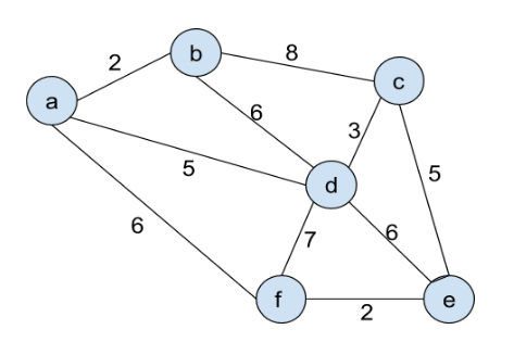
Example
Run Prim's algorithm on the input:
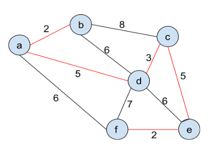
The following is the output:
Further Reading
- Section 5.2 in the textbook.
- Support page on proving adversarial lower bounds..