Recitation 12
Recitation notes for the week of November 20, 2017.
A Reminder for HW 9 Q1
Note on Timeouts on HW 9 Q1
For this problem the total timeout for Autolab is 480s, which is higher the the usual timeout of 180s in the earlier homeworks. So if your code takes a long time to run it'll take longer for you to get feedback on Autolab. Please start early to avoid getting deadlocked out before the feedback deadline.
Also for this problem, C++ and Java are way faster. The 480s timeout was chosen to accommodate the fact that Python is much slower than these two languages.
Our recommendation
- Either code in
C++orjavaOR - If they want to program in
pythonthen test on first five test cases and test for all 10 only if they pass the first five.
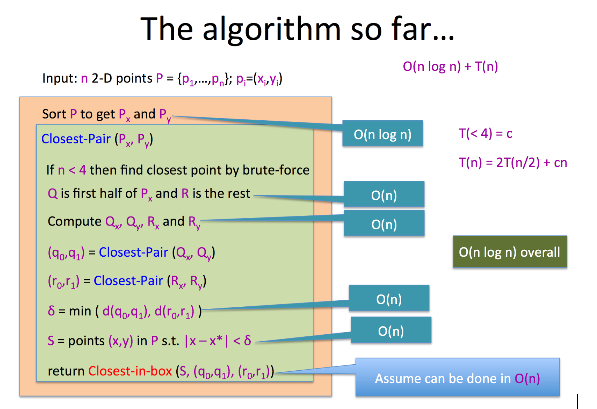
Closest Pair of Points Algorithm
The goal is to find the closest pair of points in a plane in $O(n\log{n})$ time.
Brute Force Algorithm Idea
- Just compare all pairs of points and keep track of the pair that gave the minimum distance.
- Runs in O(n^2) time.
Divide and Conquer Algorithm
Note
The algorithm we did in class assumed that the $x$ and $y$ values are distinct. Below we will outline how algorithm can be simply generalized to handle this more general case.
In the text below, names and annotations are purposefully kept the same as the lecture notes to maintain consistency.
Setup/Notation
We now setup notation that is needed to state the algorithm (and also point out what parts need to change to handle non-distinct $x$ and $y$ values.
- Let $P_x$ be the list of points sorted by lexicographic order (i.e. sort by $x$ co-ordinate first and for points with the same $x$ co-ordinate sort them by their $y$ co-ordinate), and let $P_y$ be the list of points sorted by $y$ coordinate.
Note
Note that the definition of $P_x$ is not the same as we did in class (where we just sorted by $x$ co-ordinate). Note that under the assumption that the $x$ co-ordinates are distinct, the order above matches the one we did in class.
- Let $(x^*,y^*)$ be the the middle element of $P_x$.
- We will divide the plane into two halves based on $(x^*,y^*)$. The points $(x,y)$ lexicographically smaller than $(x^*,y^*)$ goes into the left half (called $Q$ from here on) and the rest of the points go into the right half (called $R$ from here on).
Note
Note that the definition of $Q$ is not the same as we did in class (where we just made the decision based on the $x$ co-ordinate). Note that under the assumption that the $x$ co-ordinates are distinct, the order above matches the one we did in class.
- Under the more general definition of $Q$ and $R$ above, the following claim, which we say in class for the case of distinct $x$ values still holds and is left as an exercise. (The generalization is the obvious one.)
Exercise (for students)
Given $P_x$ and $P_y$ as above, compute $Q_x,Q_y,R_x$ and $R_y$ in $O(n)$ time.
Algorithm Idea
- Recursively, find the closest pair of points in $Q$ and $R$ (call them $q_1,q_2$ and $r_1, r_2$). Let \[\delta =\min(d(q_1, q_2), d(r_1, r_2)).\]
- We also need to consider crossing points between $Q$ and $R$, so we will consider a "box" which spans $x$ values from from $x* -\delta$ to to $x* +\delta$.
- If we sort the points in the box by their $y$ coordinates (note that this can be done in $O(n)$ time given $P_y$ and $\delta$), the kickass property lemma claims that any two points with a distance $< \delta$ cannot be more than $15$ indices away.
Note
The
Closest-in-boxalgorithm remains the same as the one we saw in class.
Overall Algorithm
Integer Multiplication (Re-explained)
Note
The stuff below is copied from the support page on integer multiplication.
The setup
We first recall the problem that we are trying to solve:
Multiplying Integers
Given two $n$ bit numbers $a=(a_{n-1},\dots,a_0)$ and $b=(b_{n-1},\dots,b_0)$, output their product $c=a\times b$.
Next, recall the following notation that we used: \[a^0 = \left(a_{\lceil\frac{n}{2}\rceil-1},\dots, a_0\right),\] \[a^1 = \left(a_{n-1},\dots, a_{\lceil\frac{n}{2}\rceil}\right),\] \[b^0 = \left(b_{\lceil\frac{n}{2}\rceil-1},\dots, b_0\right),\] and \[b^1 = \left(b_{n-1},\dots, b_{\lceil\frac{n}{2}\rceil}\right).\] Next, we try and reason about the $O\left(n^{\log_2{3}}\right)$ algorithm using polynomials (in one variable) .
Enter the Polynomials
We being by defining two polynomials \[A(X) = a^1\cdot X + a^0,\] and \[B(X) = b^1\cdot X + b^0.\] To situate these polynomials, we make the following observations (make sure you are comfortable with these):
Exercise 1
Show that \[a= A\left(2^{\lceil\frac{n}{2}\rceil}\right)\text{ and } b= B\left(2^{\lceil\frac{n}{2}\rceil}\right).\]
Now let \[C(X)= A(X)\cdot B(X),\] be the product of the two polynomials. Then note that by Exercise 1, we have that our final answer can be read off as \[c = C\left(2^{\lceil\frac{n}{2}\rceil}\right).\] Next, note that $C(X)$ is a polynomial of degree two and hence can also be represented as \[C(X) = c^2\cdot X^2+c^1\cdot X+c^0.\] Recall the fact that $C(X)=A(X)\cdot B(X)$ we also have \[C(X) = \left(a^1\cdot X+a^0\right)\cdot \left(b^1\cdot X+b^0\right) = \left(a^1\cdot b^1\right)\cdot X^2 + \left(a^1\cdot b^0+a^0\cdot b^1\right)\cdot X+\left(a^0\cdot b^0\right).\] By comparing the coefficient of the powers of $X$, we get that \[c^2 = a^1\cdot b^1,\] \[c^1 = a^1\cdot b^0+a^0\cdot b^1\] and \[c^0 = a^0\cdot b^0.\]
Now going back to the algorithm
The important observation is that in our divide and conquer algorithm the three recursive calls are so that we can compute $c^0, c^1$ and $c^2$. For $c^0$ and $c^2$, the recursive calls are obvious. It is for the case of computing $c^1$ that we needed the supposed "clever" identity
The Identity
\[ a^1\cdot b^0+a^0\cdot b^1 = \left(a^1+a^0\right)\cdot \left(b^1+b^0\right) - a^1\cdot b^1 - a^0\cdot b^0.\]
Now of course one can verify that the identity is correct and it works for our case. But here is another way to arrive at the identity (that uses all the polynomial stuff that we have been talking about so far). In particular consider $C(1)$. Note that we have \[C(1) = c^2+c^1+c^0.\] In other words, we have \[c^1 = C(1) - c^2 - c^0.\] Finally, note that $C(1) = A(1)\cdot B(1) = (a^1+a^0)(b^1+b^0)$ and using this in the above (along with the values of $c^2$ and $c^0$) proves the identity.
Um, why is this any better?
Finally, we give some argument to justify why the argument using polynomials is more "natural." Note that
- We needed to compute the coefficients of the polynomials $C(X)$.
- For any constant value $\alpha$ (e.g. $\alpha=1$) both $A(\alpha)$ and $B(\alpha)$ are numbers with roughly $n/2$ bits and hence $C(\alpha)$ can be computed with multiplication of two numbers with roughly $n/2$ bits.
To complete the last piece of the puzzle, we invoke polynomial interpolation . In particular, to compute the coefficients of $C(X)$ we only need the evaluation of $C(x)$ at three distinct points (each of which corresponds to multiplication of two roughly $n/2$-bit numbers). Indeed this is what has been happening above:
- First note that $C(0) = A(0)\cdot B(0)=c_0$.
- Recall we used $C(1) = A(1)\cdot B(1) = c^2+c^1+c^0$.
- Finally, we can interpret $c^2$ as $\lim_{X\to\infty} \frac{C(X)}{X^2}=\lim_{X\to\infty} \frac{A(X)}{X}\cdot \lim_{X\to\infty}\frac{B(X)}{X}$ and in a hand wavy way we can think of recovering $c^2$ by "evaluating" $C(X)$ at infinity.