BFS via examples
In which we derive the breadth first search (BFS) algorithm via a sequence of examples.
Expected background
These notes assume that you are familiar with the following:
- Graphs and their representation. In particular,
- Notion of connectivity of nodes and connected components of graphs
- Adjacency list representation of graphs
- Notation:
- $G=(V,E)$
- $n=|V|$ and $m=|E|$
- $CC(s)$ denotes the connected component of $s$
- Trees and their basic properties
The problem
In these notes we will solve the following problem:
Computing Connected Component
Input: Graph $G=(V,E)$ and a node $s$. We assume that for any $u\in V$, $Adj[u]$ is the adjacency list of $u$ (i.e. $Adj[u]=\{w|(u,w)\in E\}$).
Output: The connected component of $s$. We will assume the output is in a Boolean array of size $n$, which we will also call $R$
Next we go through a sequence of examples to build towards an algorithm that will solve the above problem. We encourage you to work on each question first and then toggle for the answer.
But if you must:
A warmup
Question 0
Let us say you have not seen the edge set $E$ but only know $V$ and $s$. In that case can you say anything about $CC(s)$?
Answer 0
$s$ is always connected to $s$. Thus, we have the following initiation for our algo:
Algorithm 0 Details
R[s]=T and R[u]=F for every u != s
For the rest of the notes, assume $E\neq \emptyset$.
Example 1
Let us now consider the following somewhat more non-trivial example of $G$:
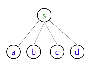
In this case, by inspection the solution is simple: we should have R[s]=R[a]=R[b]=R[c]=R[d]=T (and every other entry should be false).
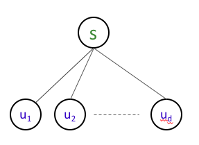
Now, let us make things bit more general. Say the connected component of $s$ is a “star” (or a tree of depth 1) graph, like so:
Question 1
How would you modify our current algo to handle this case?
Answer 1
Note that by definition, if $(s,u_i)\in E$, then $s$ and $u_i$ are connected, Thus, in the case above, we should add all neighbors of $s$ to our output. So here is our updated algorithm:
Algorithm 1 Details
                            R[s]=T and R[u]=F for every u != s

                            For every u in Adj[s]
                                Set R[u]=T
But is the above enough? As you might imagine not quite so.
Example 2
Consider the following example:
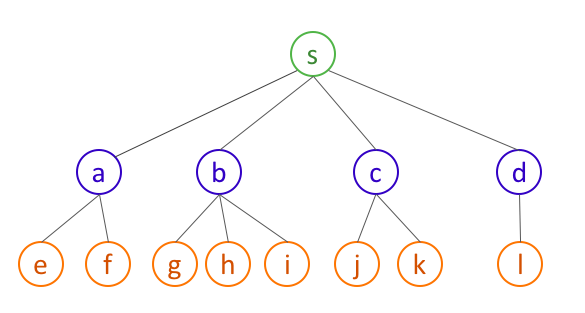
In the above example, our current algorithm will output all the green and blue nodes as the connected component, which is clearly missing the orange nodes. So the idea is that not only do we have to output all neighbors of $s$ but we also have to output all neighbors of neighbors of $s$.
Before we proceed, let us re-state our existing algorithm:
				R[s] = T and R[u]=F for every u != s
				L0 = {s}
				L1 = null

				For every u in L0 # So u will trivially be s
					For every w in Adj[u]
						Add w to L1
				For every w in L1
					R[w] = T
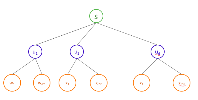
Now let us try to modify the algorithm above to work for the following more general case (basically a tree of depth 2):
Question 2
How would you modify our current algo to handle the case of a tree with depth $2$?
Answer 2
The idea is instead of just stopping at creating $L_1$, we want to look into the neighbors of $L_1$ too (which will also be in $CC(s)$). Thus, we can modify our current algorithm as follows:
Algorithm 2 Details
				R[s] = T and R[u] = F for every u != s
				L0={s} # L is for “layer”
                                L1 = null
                                L2 = null

				For every u in L0
					For every w in Adj[u]
						Add w to L1

				For every w in L_1
					R[w] = T

				For every u in L1 # Repeat for L1 what we have done for L0
					For every  w in Adj[u]
						Add w to L2

				For every w in L_2
					R[w] = T
Spot the inefficiencies
Question 4
Do you seem some inefficiencies in the above code?
The subtle one first
We start with something that is slightly subtle (but does not affect the correct of even the asymptotic runtime of the algorithm).
Question 5
When $u$ in line 5 of the Algorithm 2 is instantiated over $u_1,\dots,u_d$ (i.e. neighbors of $s$), so you see repetitions of Step 16 that is un-necessary?
Answer 5
Note that since $s$ is neighbor of $u_1,\dots,u_d$, $s$ will get added to $L_2$ multiple times.
We can get rid of the by first checking if R[w] = F before executing Step 16. However, since this does not affect the correctness of the algorithm, we let it be for now. BUT we will return to this later.
The obvious inefficiency
Note that Steps 7-12 and Steps 14-19 are essentially the same and we can use a look to write fewer lines of code, like so
Algorithm 3 Details
				R[s] = T and R[u] = F for every u != s
				i=0
				L[i]={s}

				While i<2:
					L[i+1]= null
					For every u in L[i]
						For every w in Adj[u]
							Add w to L[i+1]
							R[w]=T # There is no need to have a separate loop to do this assignment
					i++
Example 3
Now we consider the case of a general tree of depth $d$:
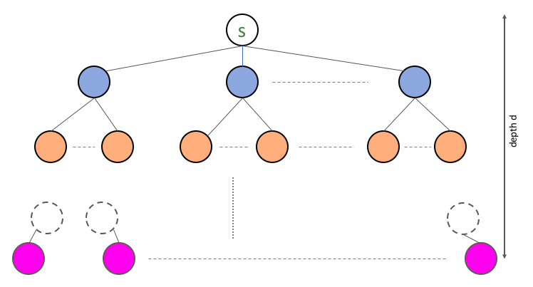
Of course our current algorithm will fail on the above (since it will not add anything beyond the orange level). However, it should now be easy to modify the current algorithm if you know the depth upfront:
Question 6
Modify Algorithm 3 to work for trees of depth $d$.
Answer 6
The idea is not to stop at the orange nodes, but then explore the neighbors of the orange nodes and then the neighbors of their neighbors etc. till you get to the pink nodes (i.e. the last level of the tree). All we need to do now is in 4 go on till depth d, like so:
Algorithm 4 Details
                                R[s] = T and R[u] = F for every u != s
                                i=0
                                L[i]={s}

                                While i<d:
                                        L[i+1]= null
                                        For every u in L[i]
                                                For every w in Adj[u]
                                                        Add w to L[i+1]
                                                        R[w]=T # There is no need to have a separate loop to do this assignment
                                        i++
Question 7 (Bonus)
What is the best runtime bound you can argue for the above algorithm? Is it $O(n)$? If not, can you make it $O(n)$? (For the analysis you can assume that each $L_i$ is a set data structure that allows for $O(1)$ insertion time.)
Answer 7
The time is dominated by the while loop in Step 6. There are $d$ iterations of the loop and since we have $|L_i|\le n$ (since these are sets), each iteration is $O(n)$. Thus, overall is $O(dn)$.
The bound above is tight: consider e.g. the case when $G$ is a “chain.”
You can improve the runtime to $O(n)$ by using an observation that we made in Example 2. In particular, if we run steps 10 and 11 only if R[w]=F, then we get $O(n)$ overall runtime. (The analysis if you have not seen it before requires a bit of care but we’ll defer this till later.)
Example 4
Now let us consider an example where $G$ is a tree plus one more edge:
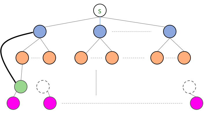
So the first thing to note that there is no notion of level since our $G$ is no longer a tree. So before we think about how to modify the existing algorithm to handle the above case, think about how one would change condition in step 6 so that we can terminate properly. In particular, let us start with the following:
Question 8
What if we check if R[u] = T for all u in V as the termination condition in Step 6?
Answer 8
This would not work as $G$ need not be connected.
This naturally brings us to the following question:
Question 9
What would be an alternate check?
Hint
What would happen to the $L_i$’s if we let the while loop in step 6 run for ever?
The obvious solution
Once you are done handling the pink nodes in the tree graph, you do not expect to get any nodes in the new layer you would aim to construct from L_d. In particular, the following seems a good fix:
Algorithm 4 Details
                                R[s] = T and R[u] = F for every u != s
                                i=0
                                L[i]={s}

                                While L[i] != null:
                                        L[i+1]= null
                                        For every u in L[i]
                                                For every w in Adj[u]
                                                        Add w to L[i+1]
                                                        R[w]=T # There is no need to have a separate loop to do this assignment
                                        i++
Question 9'
However, there is an issue with the above. The algorithm as stated will not terminate even on the tree-- do you see why?
Hint
Think back to the issue we had raised earlier in Question 5.
Answer 9
The issue is that in step 10, we blindly add w to L[i+1] even if we have already “seen it” this implies that the condition in line 6 will always be satisfied. The fix to this is what we had discussed before: before add w to L[i+1] just check if it has been already seen before. Here is the modified algorithm:
Algorithm 5 Details
                                R[s] = T and R[u] = F for every u != s
                                i=0
                                L[i]={s}

                                While L[i] != null:
                                        L[i+1]= null
                                        For every u in L[i]
                                                For every w in Adj[u]
                                                    If R[w] == F
                                                        Add w to L[i+1]
                                                        R[w]=T
                                        i++
Coming back to our example of tree plus an edge
Question 10
What happens when we run Algorithm 5 on $G$ that is a a tree plus an edge?
Answer 10
It works! Let’s look back at how the algorithm will run on this specific graph. When the algorithm is creating L[2] from L[1] (i.e. the blue nodes), then L[2] in addition to having the orange node will also have the green node in it. So effectively “pull” up the subtree rooted at the green node. The situation would look like this
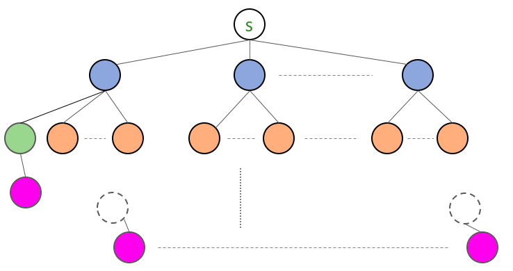
Question 11
So why is Algorithm 5 correct?
Answer 11
Basically we do not care in which order the nodes are put in: i.e. whether we discovered the green node directly from the blue node or the orange node. If we choose the latter then we would have the following situation
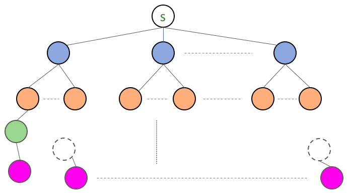
The general case
We are now ready to bite the bullet and handle the most general case. E.g. our $G$ might look something like this:
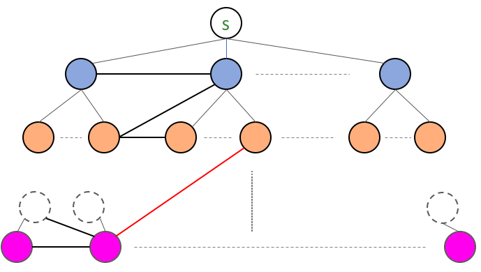
Question 12
Can you think of an example $G$ where Algorithm 5 does not work?
Answer 12
There is none! The algorithm is already enough to work on all graphs.
Question 13
Can you prove that Algorithm 5 always works?
Answer 13
You can prove this by induction (and indeed we will do so in class for a much more general algorithm that includes our current algorithm as a special case).
Question 14
Why does Algorithm 5 terminate?
Answer 14
We will show that this algorithm runs in time $O(m+n)$. In particular, it terminates! (Note that this implies that on trees, this runs in $O(n)$ time.)