Last four stages of the ML pipeline
This page contains a more detailed look at the remaining four stages of the machine learning pipeline.
-
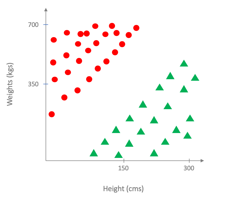
As you can probably tell, this distribution of weight and height pairs is nowhere close to being realistic. But bear with me: the point distribution is made to illustrate a broader point!
-
And even if you did, then there is no need to do prediction so setting up the whole ML pipeline is then moot!
Under Construction
This page is still under construction. In particular, nothing here is final while this sign still remains here.
A Request
I know I am biased in favor of references that appear in the computer science literature. If you think I am missing a relevant reference (outside or even within CS), please email it to me.
The ML pipeline so far
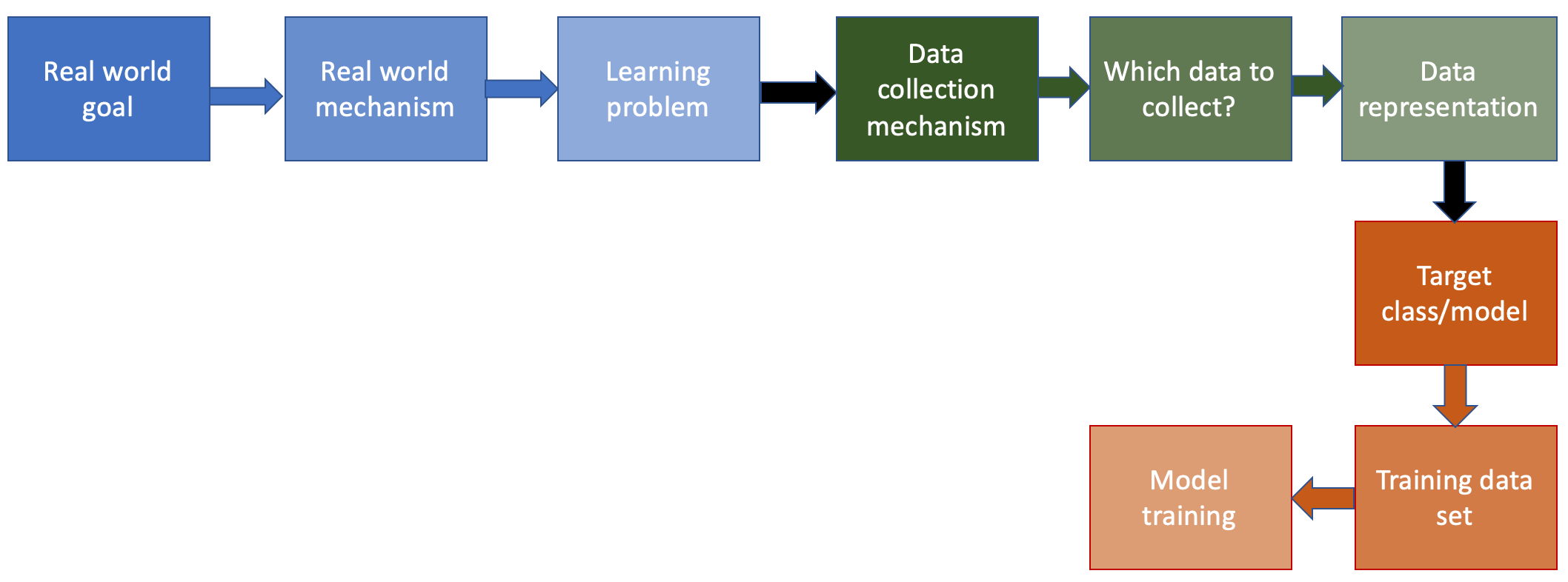
Recall that we looked at the first first six steps of the ML pipeline (all of which were specific to the problem being solved). Then we spent some time looking at the seventh step of the ML pipeline (which involved choosing the class of ML models to use). While looking at the model classes we also considered some of the remaining steps (in particular the model training step) but we will consider each of the remaining four steps in this note.
Training data set
We now move to the eighth step in the ML pipeline:
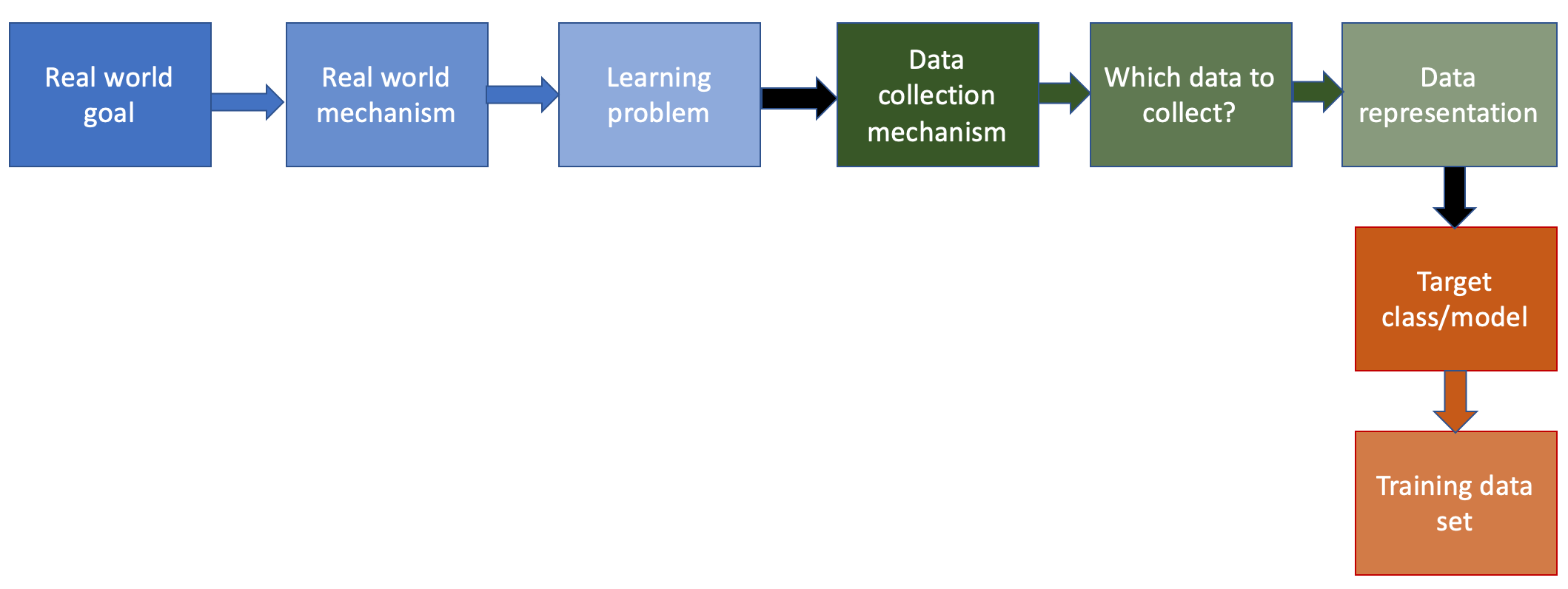
Recall that we had discussed (at a high level) how one can do model training for specific models assuming there is a training dataset. We will get back to the model training step in the next section but for now, we focus on how we choose a training dataset:
Choosing a training dataset
At this point in the pipeline, we already have access to a dataset. We now need to decide on which part of the dataset we should train our model that we choose in the previous step in the pipeline.
We start off with an obvious choice of the training dataset.
Why not use the entire dataset?
There is an obvious choice to use as a training dataset: use the entire dataset as your training dataset.
We had briefly seen before why this might not be a good idea but let us walk through an example scenario (where we will be going back to our height and weight input variable setting). In particular, assume that your "true" underlying labeling of every human looks like this1:
Changing representation of positively labeled points
We are switching how we represent a positively labeled point in the dataset from a green circle to a green triangle, with the hope that it is more accessible to readers. At a later point, we will update the earlier pictures as well. We will remove this note when that is done.
Well, the above is a bit too extreme, so perhaps the following is a more "realistic" ground truth (or perhaps-- and this might be valid in some other situations-- the correct underlying distribution is like above but when we try to measure it, we get some erroneous measurements, which can also lead to the situation below):
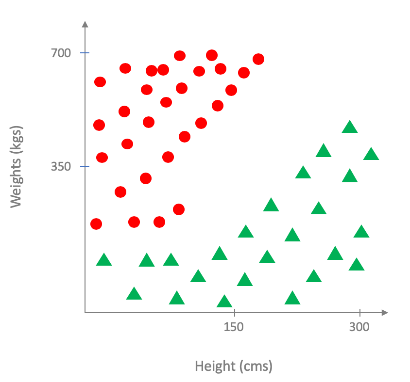
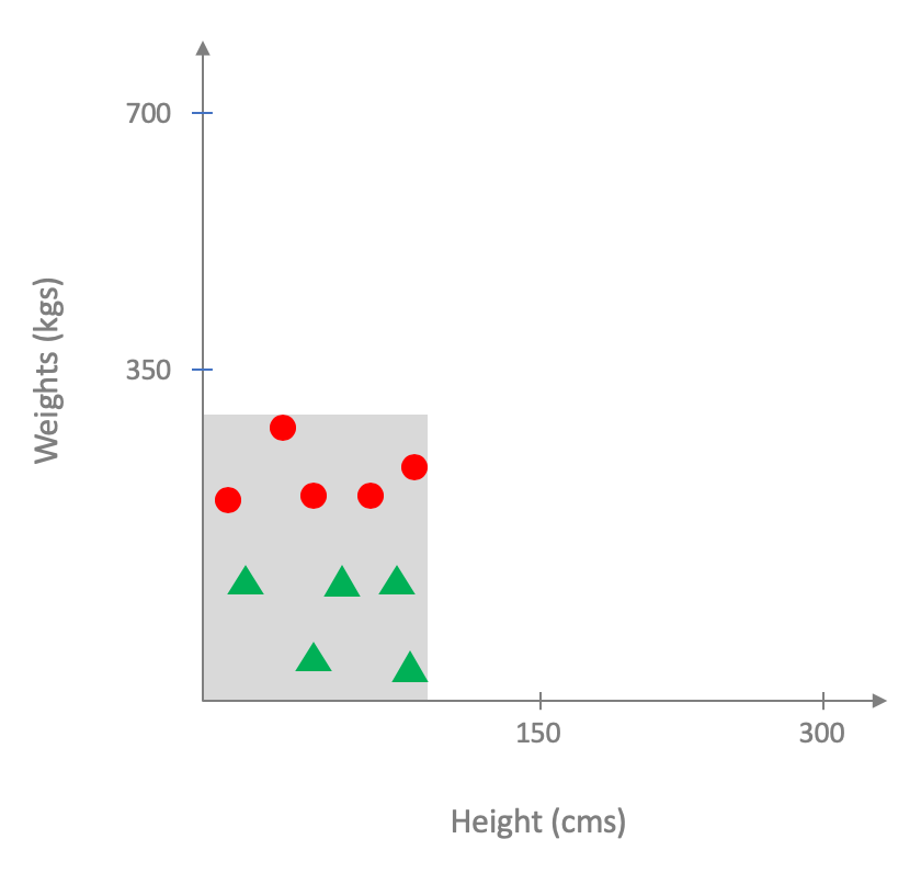
Now it is very unlikely (if not impossible) that you will have the information on weight, height and risk of heart disease for all humans on the planet2. What you will have access is to a subset of the underlying distribution, which forms your dataset, like so (the dataset region is shaded in gray):
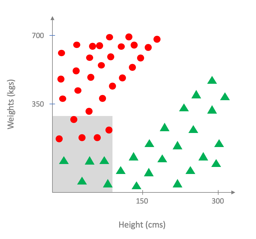
Thus, for the purposes of training your model, this is what it would look to your ML pipeline:
Focus on linear models
For simplicity, we will assume that we have chosen the class of linear models in our previous step. This will make the pictures easier to draw etc.
However, it turns out that for the example above, the situation will exactly be the same even if we had picked the decision tree or neural network model. If you are not convinced with this, figure out why as an exercise!
In other words, if we were to use the entire dataset as our training dataset, our next step of model training will get the above as its input and will then output the following as the optimal linear model that fits the dataset:
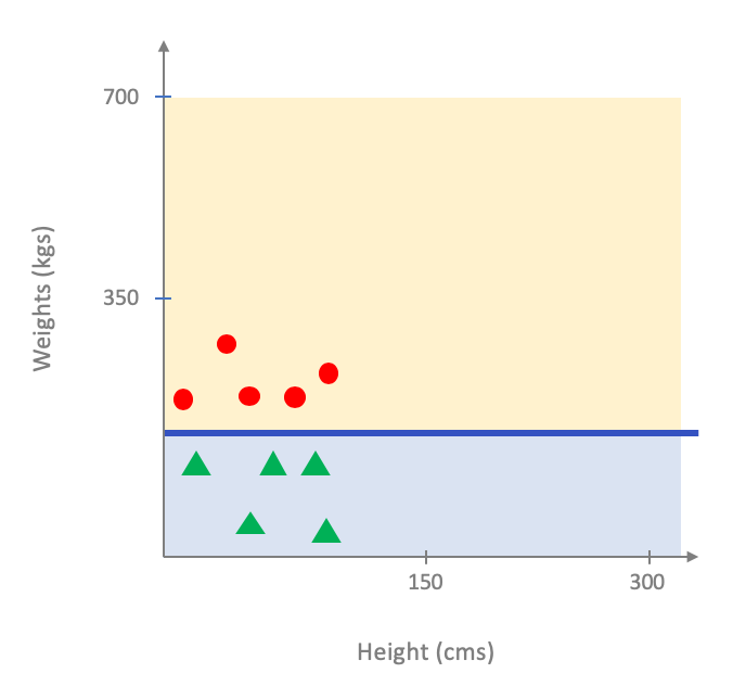
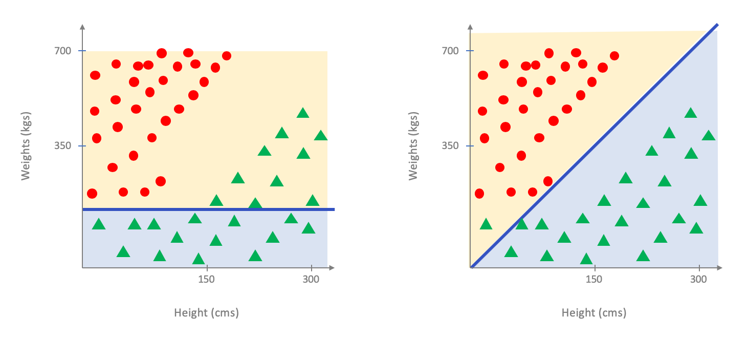
As you probably see the above is not a good fit for the entire population. In case you are not convinced here is a comparison on how the model above does on the entire population (figure on the left below) vs. an optimal linear model for the entire dataset (figure on the right below):
Now, you could protest that the above is a made up scenario and what about the following:
What IF our dataset was a true random sample of the ground truth
Now consider the following scenario: what if our dataset is a true random sample from the underlying distribution? In this case, we can actually guarantee that the optimal linear model for the random sample will be very close to the optimal linear model for the entire population (assuming there are enough random samples in the dataset). We will not go into this but the mathematical buzzword that makes this work is that the VC dimension of linear models is constant (in case you care it is $3$).
At this point you might be thinking: wait, does not the above mean that we are done? Well, not quite. Let me quote the relevant from above:
What if our dataset is a true random sample from the underlying distribution?
The issue is that assuming that we have access to a truly random sample of the underlying distribution is (literally) a big if. In fact, in many real life scenarios, where applications of ML can hay-wire happens precisely because we forget the big if.
Hopefully by now you are (somewhat?) convinced that we should not use the entire dataset as the training dataset. But then the question remains: which subset of the dataset should we use? We tackle this next (and then we will be done with our discussion on the eighth steps of the pipeline).
Which subset of the dataset should we use?
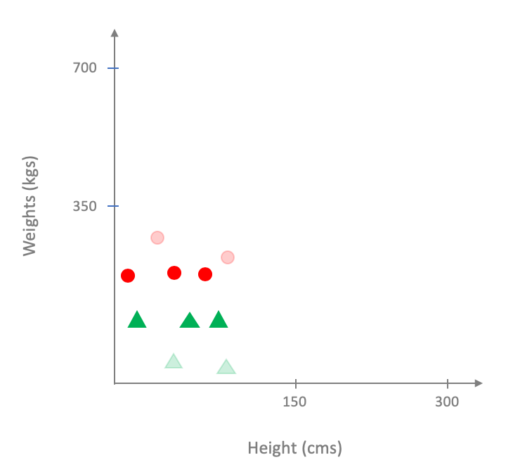
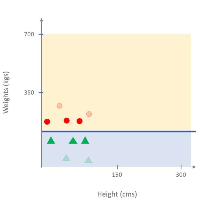
We now use the pesky question of which subset of the dataset to use for model training? It is not too hard to see that the choice of the subset can have very strong effect on the final output. For example, consider the case when we pick the following subset (where the points we did not choose are more transparent):
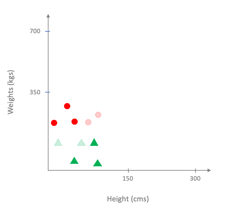
On the other hand if we picked the following subset:
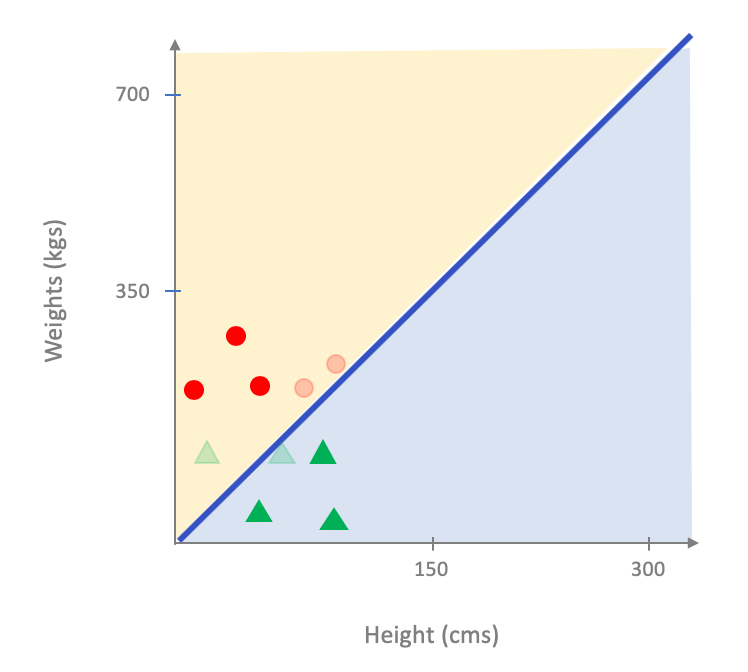
How do we pick the best subset?
So the pesky question now becomes: how do we figure out the "best" subset?
The problem is that answering this question is just not possible: to figure out the best possible subset, we need to know the underlying ground truth. But the whole reason we are doing prediction is that we do not have access to the ground truth in the first place. So how do we get around this?
The answer is that we punt and "guess." In other words, we do the following:
- Figure out what fraction of dataset we want to use to obtain out training set. I.e., we first figure out the size of the training set relative to the dataset. In the above examples, the training sets were of size $6$ while the dataset had $10$ points in it-- i.e. we picked $60\%$ of the dataset as the size of our training set.
- We then pick a random subset of the size determined in the previous step and use that as the training dataset.
We would like to note that we talked about two kinds of random subset/samples and it is worthwhile to see how they are different.
Two kinds of randomness
Now is a good time to recap the two random subsets of data we talked about.
The first random subset we considered was a random subset of the ground truth. This subset has very nice theoretical properties is something we do not have access to in real life.
The second random subset we considered was a random sunset of the given dataset. Thus, in this case we are looking at a random subset that we can always construct.
In other words, we can construct a random training dataset from a given dataset but in general we cannot hope to create a random dataset (from the ground truth). However, in many scenarios where applications of ML go awry, it is assumed that the dataset is actually a random dataset (from the ground truth). We will come back to this point later on in the course.
Beyond random training datasets
As it turns out picking a random training dataset from the given dataset is not the only way to construct training dataset. For example, in many situations, one might construct multiple training datasets and use those to get multiple models. Then one could pick the "best" model based on how well these models do on the test dataset. A well-known example of this is cross validation . However, to keep our discussion simple, we will not consider these more (though not that much) complicated methods to create training (as well as testing) datasets.
Now that we have created the training dataset, we have to train our model on the training dataset, which we consider next.
Model training
We now move to the ninth step in the ML pipeline:
We have already looked at the model training step for linear models, decision trees and (very briefly} for neural networks. However in all of these cases, we do not know of very efficient way to train models. We mentioned the gradient descent algorithm that is used as a heuristic to solve this step for general model learning. The aim of this section is to motivate and give some of the main ideas behind gradient descent.
Linear model in one variables
Even though we know how to efficiently solve the training problem for linear models in one variable, we will focus on this special case of linear model in one variable to explain the algorithm that works for other models as well (since it makes it easier to explain the relevant concepts).
We start with the natural error function that we used to evaluate a given model-- i.e. the number of mistakes it makes on a training set of $n$ points. Let us visualize this error function next:
Minimizing the number of mis-classified errors
We will use the following training dataset with $n=9$ points for our discussion in this section:

Recall that to define a linear model in one variable we need to fix the threshold $b^*$ along with which side get the positive values.
For the time being let us consider linear models that colors $b$ values to the right of $b^*$ to be blue. Then for each value of $b^*$ in the range of acceptable values one could plot the number of points the model mis-classifies. In particular, for the example above, we will have the following behavior (where we present a "bar chart"):
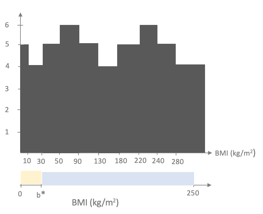
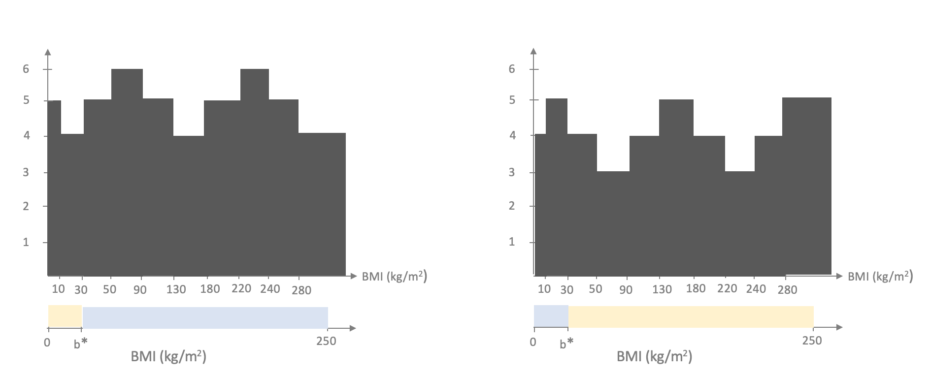
Thus, the overall optimal linear model is to pick the threshold in $[50,90)$ or $[220,240)$ such that the value left of the threshold gets colored blue.
Let us now consider the "landscape" of the number of misclassified point but just plotting the number as a "line plot":
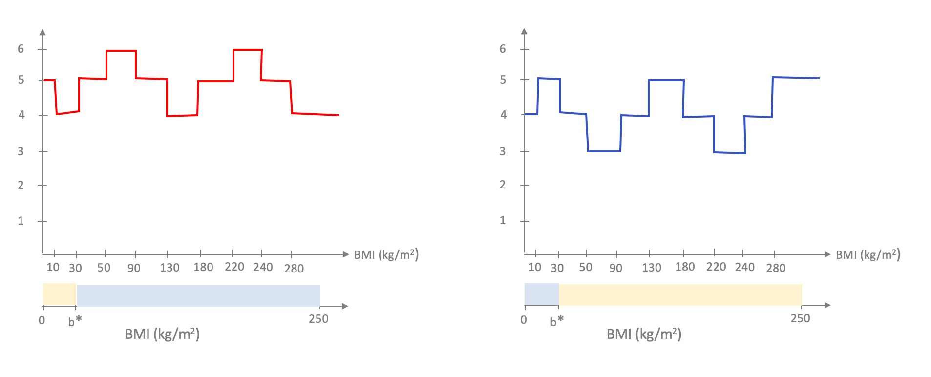
The plot looks like a "staircase" and this is something that we used to our benefit for the special case of learning linear model in one variable and is also the reason why generalizing to larger number of input variables becomes hard. First, recall that we note that we only need to consider the "corner" values in the staircase and indeed there are at most $n$ corners that we need to consider and we exploited this to perform training in roughly $n$ steps. It turns out that one can also only look at corners when we have $d$ input variables but in that case we have to consider $n^d$ corners, which quickly becomes infeasible.
One could hope that perhaps we could avoid checking all the corners. Unfortunately, this is unavoidable. So we seem "stuck"-- how do we get around this issue?
Other loss functions
As mentioned above, while using the number of misclassified points as the error metric during the model training phase is a natural choice, this leads to inefficient model training (especially when we are considering more than one input variable, which is in most cases in real-life applications of the ML pipeline). This has led to having a separate loss function that is related to the number of misclassified points but the function is "smoother" than the accuracy measure we have seen so far (which makes it easier to efficiently optimize for).
We first consider a common loss function and then use that to illustrate the main ideas behind the main algorithm (gradient descent ) that is used for model training (pretty much across all model classes. We will then see another common loss function and conclude with some observations on what we lose when we change our loss function.
Loss function
For simplicity, we will define a loss function for linear models on one variable (though the definition is fairly easy to generalize to other settings). Recall that the training dataset is a collections of input value and label pairs: i.e. $(b_1,y_1),\dots,(b_n,y_n)$. In the example used above (with $n=9$) the training dataset is \[(10,-1), (30,1), (50,1), (90,-1), (130,-1), (180,1), (220,1), (240,-1), (280,-1).\]
The loss function $L$ for linear model $\ell$ is defined as follows. For any $1\le i\le n$, $L(\ell,i)\ge 0$ is defined to be the loss that the model $\ell$ incurs for the pair $(b_i,y_i)$. For example, for misclassification, the loss function is defined as $0$ if $\ell(b_i)$ is the same as $y_i$ and $1$ otherwise. Bit more mathematically:
\[L(\ell,i)=\begin{cases}
0 & \text{ if } \ell(b_i)=y_i\\
1 & \text{ otherwise }
\end{cases}.\]
The overall loss for the model $\ell$ is to just sum up the losses for each of the $n$ points. In other words,
\[L(\ell) = \sum_{i=1}^n L(\ell,i).\]
For the example of misclassification the above is exactly the same as the total number of mis-classified points.
Square Loss function
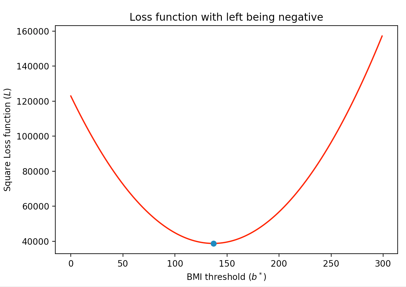
For simplicity, let us consider linear models where the values to the left of the threshold value of $b^*$ get the yellow color. Recall that this means that the linear model is defined as \[\ell(b)=\begin{cases} -1 & \text{ if } b\lt b^*\\ 1 & \text{ otherwise} \end{cases}. \]
The idea in the square loss function is that mistakes for $b_i$ values that are farther away from the threshold value get penalized more (note that in the loss function that counts the number of misclassified points, the loss function counts all misclassification as the same). For the dataset from earlier (which we repeat below for convenience):

Click here to see a more precise definition of the square loss function
We begin by re-defining the linear model (in a more succinct manner. Convince yourself that a linear model with threshold value $b^*$ is exactly the same as the function
\[\ell(b) = \textsf{sign}(b-b^*),\]
where the sign function is defined as
\[\textsf{sign}(x) = \begin{cases}
-1 & \text{ if } x\lt 0\\
1 & \text{ otherwise}.
\end{cases}
\]
Now note that the loss function corresponding to the number of misclassification can equivalently be defined as \[L_{\text{accuracy}}(\ell, i) = \left(\frac{y_i-\textsf{sign}(b_i-b^*)}2\right)^2.\] If you do not see it, spend some time and convince yourself!
The idea behind the square loss function is to simply drop the sign function in the above, i.e. \[L_{\text{sq}}(\ell, i) = \frac 14\cdot \left(y_i-(b_i-b^*)\right)^2.\]
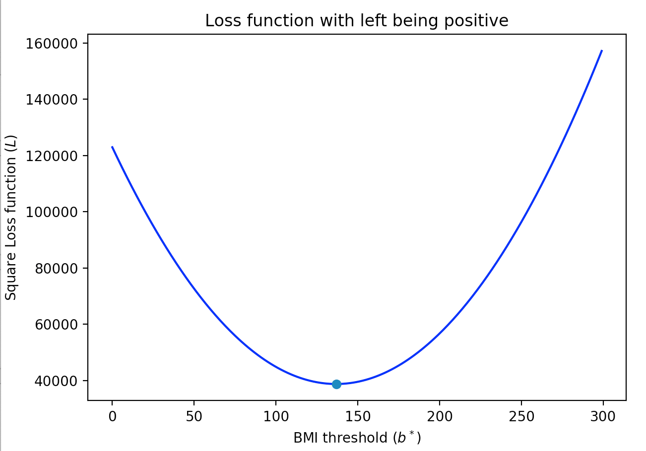
For completeness if the linear model colors points to the left of the threshold value as blue then the resulting total loss function would look like this:
Towards gradient descent
We will not delve much into the technical details of gradient descent but we will go over a high level overview of the algorithm. So recall where we are-- our (square) loss function looks like this:

A 1000 mile view of gradient descent is that if one were to skate on a half-pipe (assuming the skater does not push themselves so hard that they cross over), then eventually the skater will stop at the lowest part of the half-pipe, like so
Coming back to our square loss function, the situation is something like this (gif generated via ezgif ):
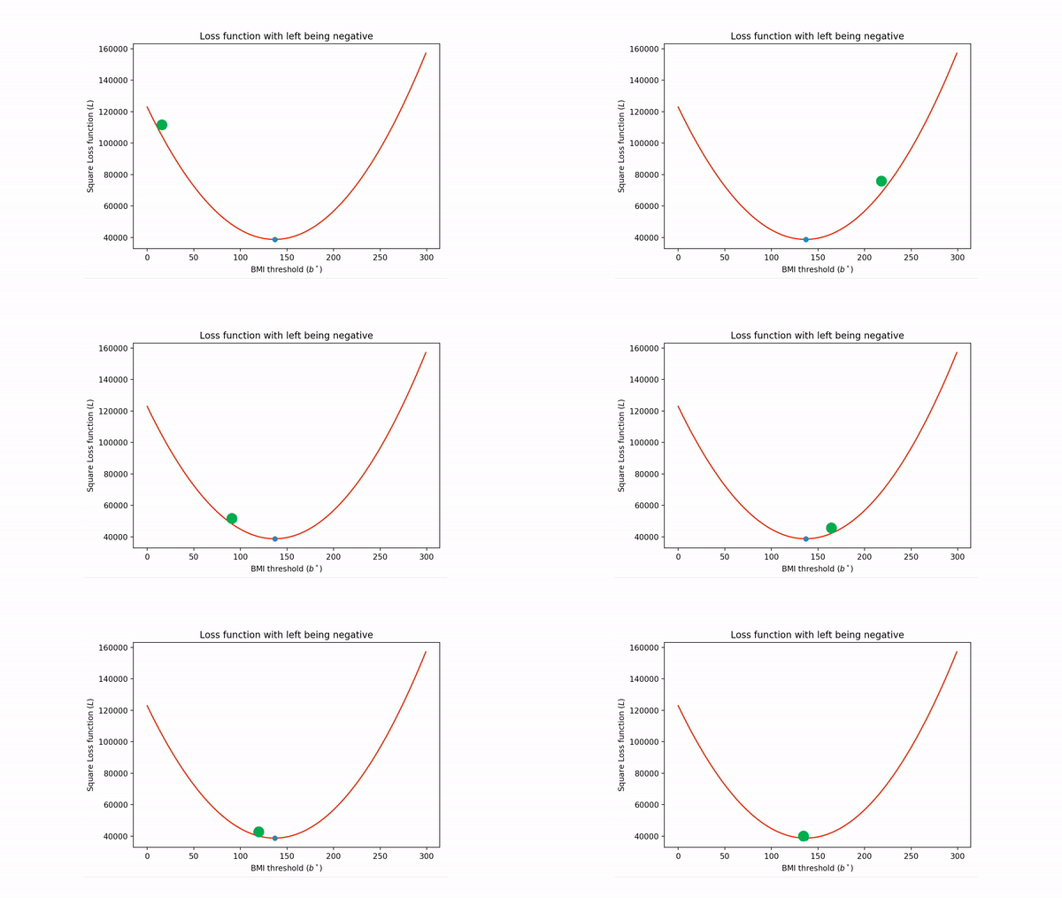
If we were to carry on with the above physical interpretation for a bit longer then the algorithm basically is
- Put the green ball at an arbitrary point on the the loss function.
- Then let "gravity" drag the ball to bottom and then it "momentum" carrying it beyond the minimum point and this process creates a back and forth movement.
- Eventually "friction" slows down the process and the ball "settles" down at the minimum point (and so after the ball spots we have found our unknown minimum point).
Unfortunately, during model training on a dataset, we do not have gravity or friction. However, fortunately, we do have mathematical analogues which roughly correspond to the tangent and derivative (both of these information are captured by gradient -- which is also defined for more number of variables-- and hence the "gradient" in gradient descent).
Gradient Descent
We first recall the definition of a tangent of a point-- it is the line that just touches that point. Further, the tangent naturally defines two direction, as we explicitly point out for the green purple points on the square loss function above:
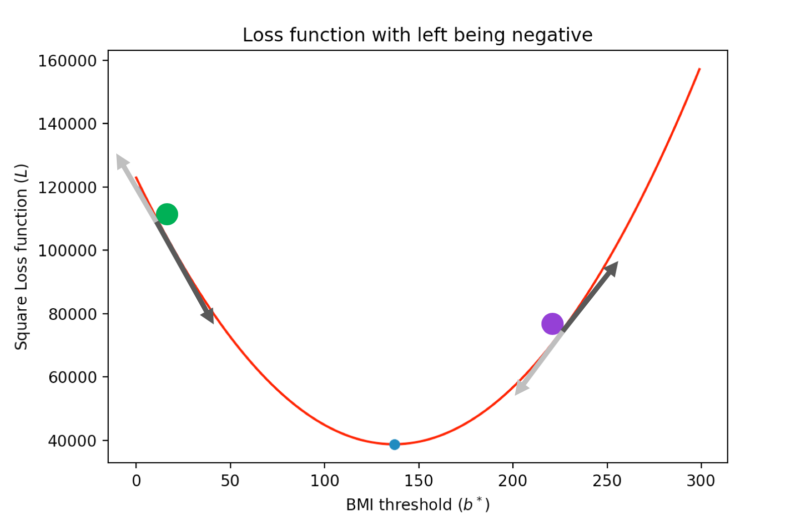
Of course for the green point we want to take the darker direction while for the purple point we want to take the lighter direction. It turns out that this information is encoded in the sign of the derivative (in the picture above if the darker arrow points down then the derivative is negative and if the darker arrow points up then the derivative is positive) of the function at the corresponding point! In other words, we can use the sign of the derivative to play the part of gravity-- if the derivative is negative then the "gravity" is in the direction of the derivative and if the derivative is positive then the "gravity" is in the opposite direction.`
The derivative is all you will need
So we have found the analogue of gravity in the sign of the derivative but we need some notion of "friction" so that one "slows" down as one comes closer to the minimum point. It turns out that this follows from the value of the derivative. In particular, the derivative is zero at the minimum point and it becomes progressively smaller (larger) as comes close (goes far respectively) to the minimum point, like so
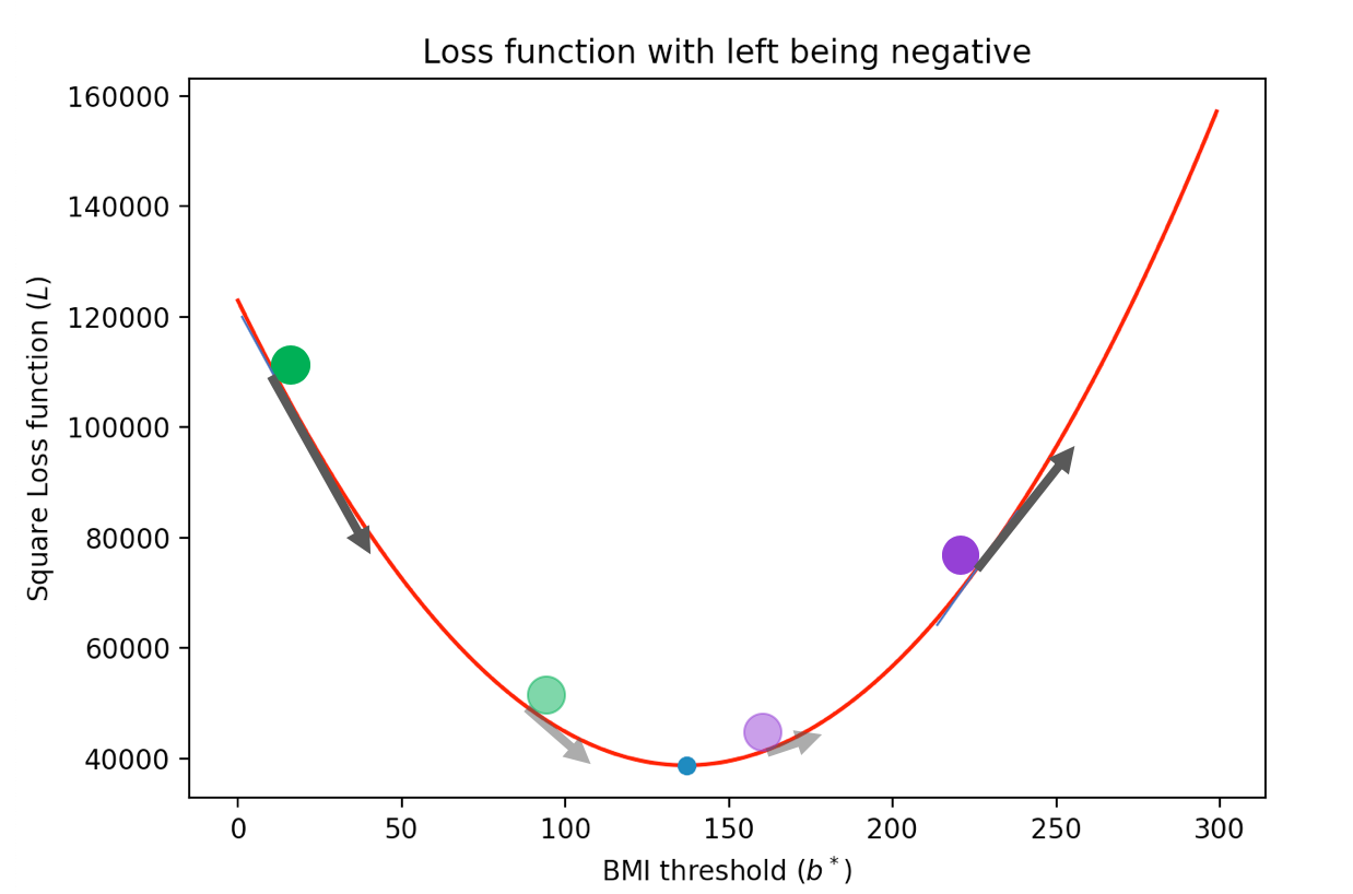
Given this the update rule is simple. Let $b_{\text{curr}}$ be our current "guess" for the threshold value. Let $L'(b_{\text{curr}})$ be the value of the derivative of the total loss function at that point (in the image above the derivative value is denoted by the length of the arrow and the sign is positive if the arrow points up and negative if the arrow points down). Then we want to increase the value of $b_{\text{curr}}$ when the derivative is negative and decrease the value of $b_{\text{curr}}$ when the derivative is negative. This suggests the following very natural rule (where $b_{\text{new}}$ denotes the new value we want to check next): \[b_{\text{new}}:= b_{\text{curr}} - L'(b_{\text{curr}}).\] In other words, we assign the new value $b_{\text{new}}$ to be the quantity $b_{\text{curr}} - L'(b_{\text{curr}})$.
It turns out that in general, we want to also control how "far along" the derivative we want to move. Towards this end we use a learning parameter which is just a positive value $\gamma\gt 0$ such that the update rule becomes:
\[b_{\text{new}}:= b_{\text{curr}} - \gamma\cdot L'(b_{\text{curr}}).\]
Overall model training algorithm
We now have enough to present the final gradient descent based model training algorithm:
Gradient Descent based model training algorithms
                                // There is only one input variable b
                                // Input: Training data set (b1, y1), ...., (bn, yn)
                                // Input parameter: learning parameter gamma

                                //Compute some functions
                                Compute the loss function L from training dataset
                                Compute the derivative function derivL of L


                                /*Gradient Descent part starts now*/

                                Initialize b* to an arbitrary value

                                while stopping condition not satisfied //Stop if  L(b*)is small enough or too many iterations

                                    delta = derivL(b*)
                                    update b* to b* - gamma*delta

                                Output the current value of b*
On some of the steps
The above description of the algorithm does not specify how some of the steps will be implemented. We briefly consider them here:
- Computing
LandderivL. It turns out that for the square loss function (and many other loss functions that are used in practice), there is a closed form expression for the total loss function $L$ (as well as its derivative ) in terms of the training dataset points (and their labels). stopping condition. Typically one of two check are made (or sometimes we continue till either one is satisfied) when deciding when to stop:- There is a pre-determined bound $T$ on the number of iterations of the loop on line 14. The loop stops once at least $T$ iterations have been executed.
- There is loss bound of $\epsilon$. The loop stops is one has $L(b^*)\le \epsilon$.
- Picking the learning parameter
gamma. There are some heuristics that are used in general. For certain loss functions one mathematically pick the value ofgammabased on the choice of $T$ and $\epsilon$ from the previous step.
When does it work?
Gradient Descent seems like such a simple algorithm-- does it really work? Or can we prove that it works?
If I had just stated the description of the algorithm up front, then y'all might not have believed it. However, it turns out that the gravity/friction and derivative/gradient analog actually can be made to provably work. The question then is for what kind of loss functions can we prove that gradient descent always work (i.e. it always terminates at a minimum value in a reasonable number of steps)?
Convex (loss) functions
It turns out that the gradient descent always works for loss functions that are convex . Informally, these are functions that look like a half-pipe and have a global minimum at the "bottom." Bit more formally, a loss function is convex if the line connecting any two points on the function is contained "inside" the function. For example, for the square loss function that we have seen so far, the line connecting the green and purple is "above/inside" the loss function:
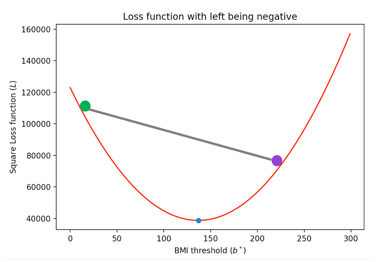
There is a huge body of work on optimizing function that are convex, called convex optimization , which is the computational workhorse around which most of ML is built. The details of convex optimization, while very fascinating, is unfortunately outside the scope of this course.
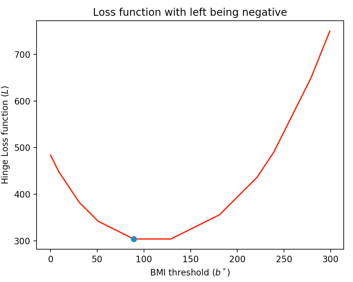
We will however, given another example of a well-known convex loss function-- the hinge loss function .
The idea behind the hinge loss function, like in the square loss function is that mistakes for $b_i$ values that are farther away from the threshold value get penalized more (note that in the loss function that counts the number of misclassified points, the loss function counts all misclassification as the same). For the dataset from earlier (which we repeat below for convenience):

Click here to see a more precise definition of the hinge loss function
We begin by recalling the re-definition linear model:
\[\ell(b) = \textsf{sign}(b-b^*),\]
where the sign function is defined as
\[\textsf{sign}(x) = \begin{cases}
-1 & \text{ if } x\lt 0\\
1 & \text{ otherwise}.
\end{cases}
\]
Now note that the loss function corresponding to the number of misclassification can equivalently be defined as (and this is different for how we looked at the loss function): \[L_{\text{accuracy}}(\ell, i) = \frac 12\cdot \left(1-y_i\cdot\textsf{sign}(b_i-b^*)\right).\] If you do not see it, spend some time and convince yourself!
The idea behind the hinge loss function is to simply drop the sign function in the above and to penalize "positive" loss more than negative loss: \[L_{\text{hinge}}(\ell, i) = \max\left(0,1-y_i\cdot\textsf{sign}(b_i-b^*)\right).\]
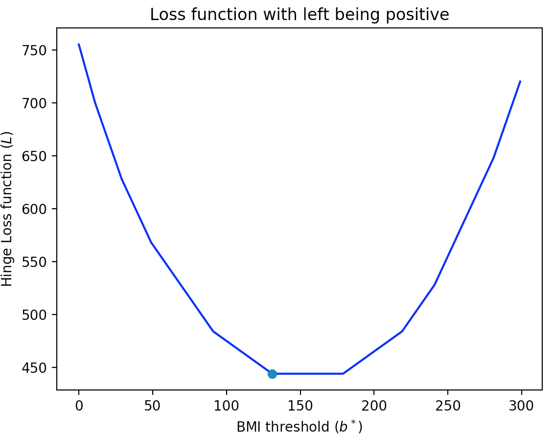
For completeness if the linear model colors points to the left of the threshold value as blue then the resulting total loss function would look like this:
What about non-convex (loss) functions?
A natural followup question is what happens when gradient descent is run on non-convex function. It is not hard to show that there exists non-convex loss function where gradient descent might get stuck in a "local" minima instead of a getting to the global "minima". E.g. in this non-convex loss function (convince yourself that this is not a convex function!):
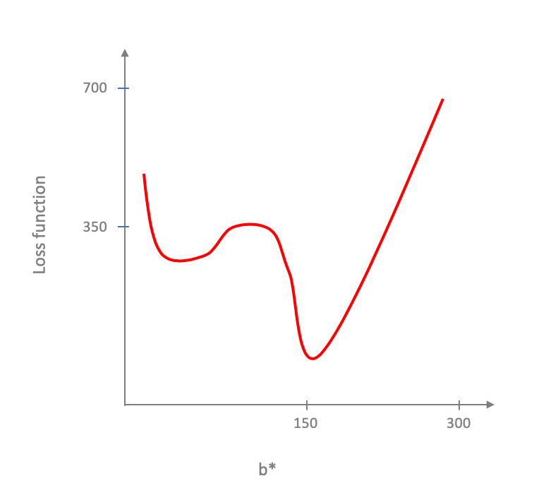
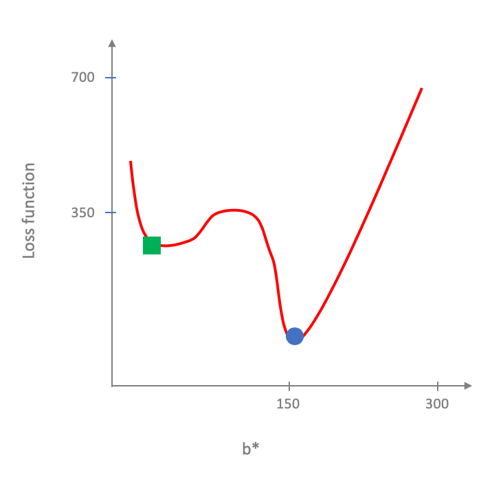
It is not too hard to see that is the gradient descent starts at the wrong place then it can get stuck at the green square.
However, it turns out that in practice, gradient descent (or rather some of its generalizations) tend to work surprisingly well for non-convex functions. Our (mathematical) understanding of this phenomenon, at the time of the writing of these notes, is pretty poor. In case you are interested, here are some (fairly) technical slides on non-convex optimization from an advanced ML course by Chris De Sa .
Moving beyond one variable
We have on purpose kept our discussions to the case of one variable but gradient descent works on convex function in more than one variable. Here is a nice animation by Alykhan Tejani of gradient descent on a convex loss function on two variables (where the goal is still to fit the best linear model-- though not for binary classification but for the related problem of linear regression ):
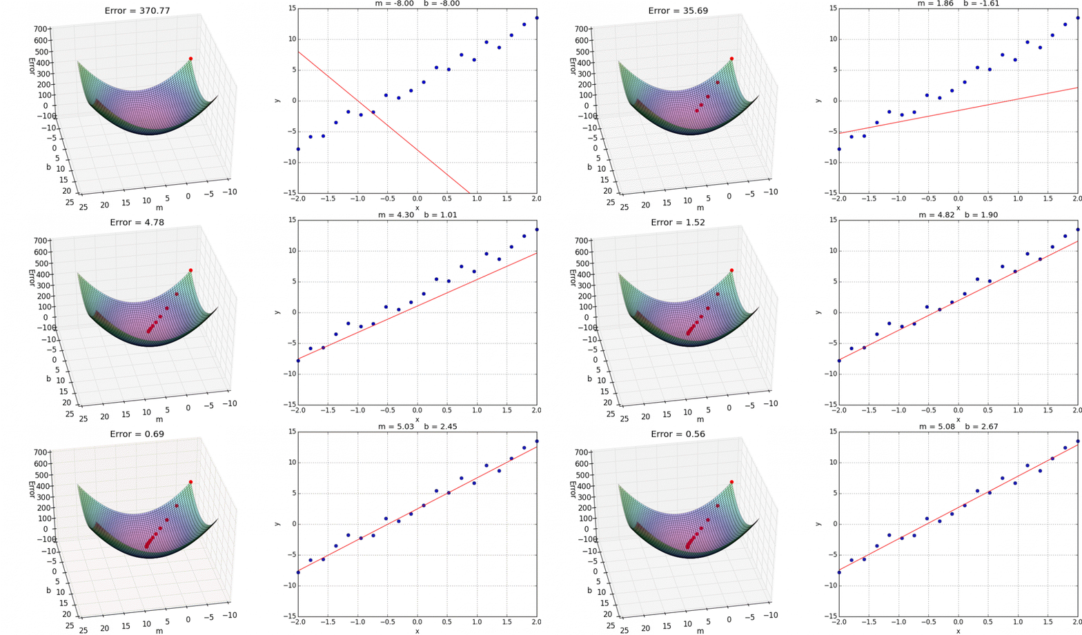
For other examples of animation for gradient descent on two (or more variables), see e.g. here and here .
What did we lose and some generalizations
Let us come back from our discussion on gradient descent to why we got here in the first place. In particular, we started off by replacing the (non-convex) loss function of counting the number of misclassification errors by convex functions like the square or hinge loss function. For these latter functions, we learned that gradient descent provably works in finding the minimum threshold we were looking for (and fairly efficiently-- though we have not really justified the claim on efficiency). So the question becomes: we have gained in efficiency in model training-- have we lost something in the process?
What did we lose?
Recall that ideally we would still have liked to use the total number of misclassified points as our loss function (since that is what we will end up using as our main way to measure accuracy during the last step in the ML pipeline). In other words, we used the square/hinge loss as a proxy for the actual loss function we really wanted to use.
Perhaps we can get lucky and somehow get the optimal threshold value for our ideal loss function. Now would be good time to tell y'all about the exact minimum threshold value that we get from the four convex loss functions we have seen so far:


The minimum threshold values for the four loss functions (in order are): $137, 137, 89$ and $131$ respectively.
Exercise
Figure out how many points are misclassified if one uses the minimum threshold values as above. Do any of them give the smallest possible number of misclassified points? If not, how close do they get?
Hint: None of them get the absolute minimum of three classification errors.
Hence, while we gain in efficiency, we lose in getting the actual optimal model. However, it turns out that in real life using these proxy convex loss functions seems to work fairly well. However, in practice one needs to look at generalizations of gradient descent such as stochastic gradient descent , though again, doing these topics any justice is outside the scope of this course.
We are now done with our discussion on the model training steps. Next, we move to the second last step of the ML pipeline-- testing the model we just learned in this step.
Prediction on test dataset
We now move to the tenth step in the ML pipeline:
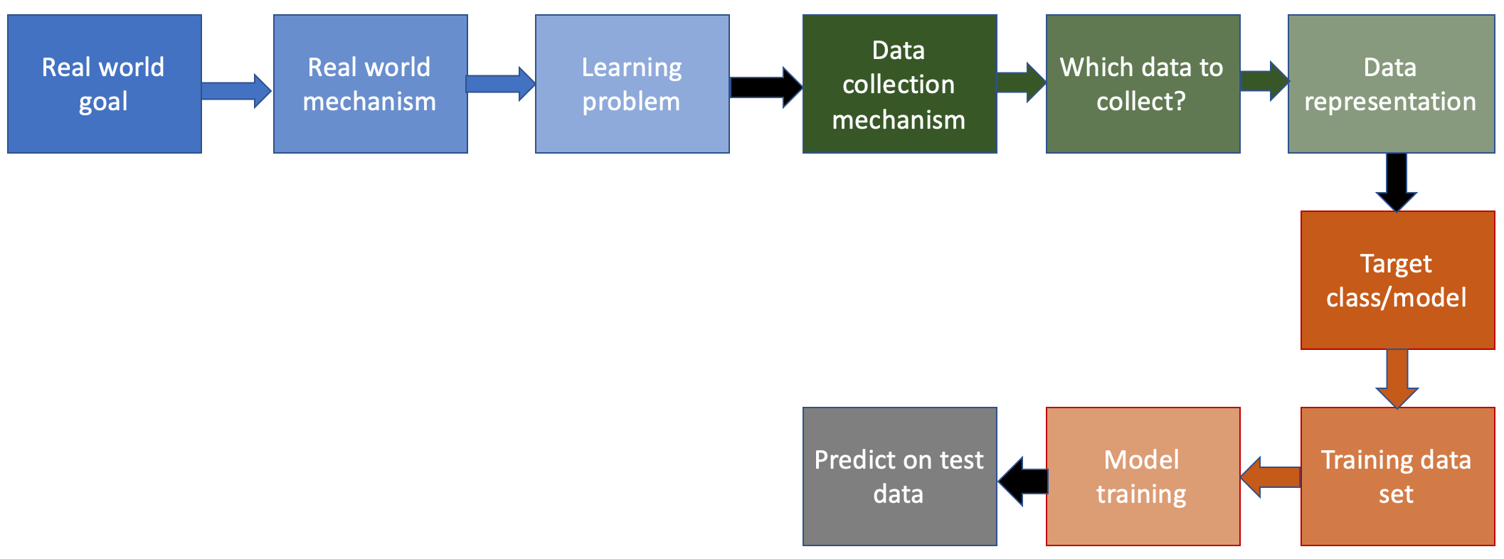
Actually as it turns out that we have already covered most of material here earlier. In this step we need to decide on two things (recall that at this point we already have our hands on a model from the previous model training step):
- Figure out a testing dataset from the original dataset collected after the end of the sixth ML pipeline step with say $N$ test data points.
- Predict the label on each of the $N$ test data points using the model we currently have.
We consider these two steps in reverse order:
Predicting on testing dataset
When considering model classes, we have already considered the problem of prediction (e.g. see our earlier discussion on efficient prediction for linear models, decision trees and neural networks). Then doing prediction on the $N$ test data points is simple:
- Run the prediction algorithm for the given model on each of the $N$ test data points and record the predicted label.
Thus, the overall time taken by this step is $N$ times the time taken for one prediction, which overall is reasonable if one prediction can be done efficiently.
Picking the testing dataset
Actually, this part is easy: since we have already picked a subset of the original dataset as the training dataset, pick the rest as the testing dataset.
If you do something bit more fancy than picking a random subset of the dataset as the training dataset (such as cross validation), then picking the testing dataset also becomes bit more interesting, but we will not explore this option in this course.
We are almost done with the ML pipeline! Finally, we evaluate how well the chosen model does on the testing dataset.
Evaluate error
We now move to the final step in the ML pipeline:
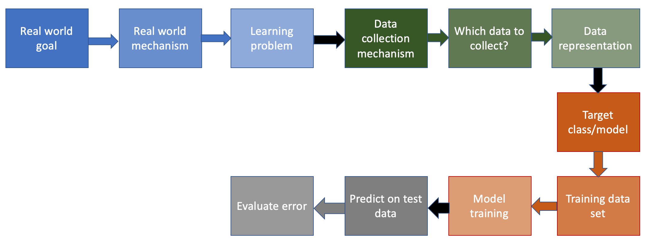
At this step, we have for each of the $N$ datapoints in the testing dataset the label that our chosen model gives to those points. The last step is to evaluate the overall error of our chosen model on the training dataset and we do so with the most obvious option:
Measuring accuracy
For each of the $N$ training dataset points, check if the model classifies it correctly according to its original label in the dataset. In other words, we count the number of misclassification error.
We should note that by no means this is the only notion of accuracy (and indeed in the next part of the course we will explore more such options) but this is definitely the most commonly used one so for now, we will just mention this option.
Why did we use a convex loss function in the model training phase?
One question that might be troubling you is why we picked the number of misclassified points in the testing dataset as our notion of final model error but did not use the same notion of number of misclassified point as the loss function in the model training phase?
We have already talked about this but it bears repeating-- the difference is due to efficiency considerations. Figuring out the optimal model using the number of misclassified points does not have any efficient algorithms, which is why we used a convex loss function for which we can find an optimal model using gradient descent. On the other hand, for evaluating the error of the chosen model on the testing dataset, we only need to run $N$ predictions, which is efficient.
Coming back to accuracy
See the following twitter post by Geoffrey Hinton (one of the leading figures in deep learning):
Suppose you have cancer and you have to choose between a black box AI surgeon that cannot explain how it works but has a 90% cure rate and a human surgeon with an 80% cure rate. Do you want the AI surgeon to be illegal?
— Geoffrey Hinton (@geoffreyhinton) February 20, 2020
Exercise
What would be your answer? Justify your answer :-)
Stepping back a bit, what do you think of (the framing of) Hinton's question?
A digression: A Vizier exercise
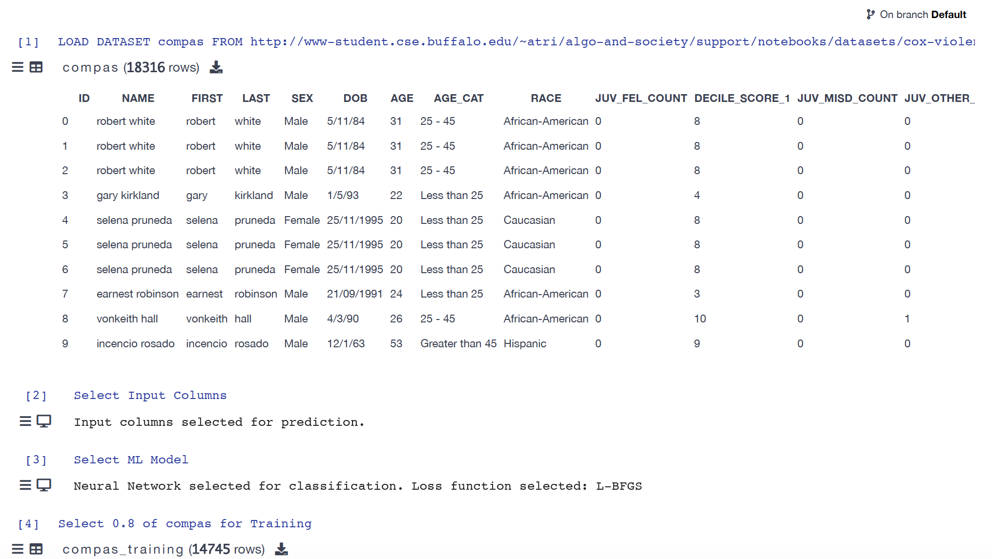
Before we move on, let's use Vizier to get a sense for how changing various parts of the ML pipeline changes overall accuracy:
Load the notebook
Log on to Vizier server (if you are registered in the class . The click
on the projected titled ML pipeline - Choosing Loss Function, which would look like this:
Increase the accuracy
Without changing the set of input variables (or target variable) and not changing the training or testing dataset, how close can you get the accuracy to $100\%$?
Another Exercise
Create an end-to-end ML pipeline using the adult dataset where the target variable is Over-50K. Your goal should be to maximize the final accuracy subject to the constraint that you cannot use more than six input variables.
If you are not registered in class
Vizier currently does not have a public online server: it is something in the works. In the meantime, we will try and put the notebooks available to download and used if you have Vizier installed on your machine: more details coming soon.
Next Up
Finally, we are at a place to put society back into the ML pipeline. In particular, we will consider (some) notions of fairness next especially with regard to the outcomes of an ML binary classifier.